Bonsai LLM Benchmark: Jetson Orin Nano Super 8GB
5 Bonsai-family 1–1.58bit LLMs benchmarked across 4 power modes on Jetson Orin Nano Super 8GB. 25W sweet spot: 47–48% more tok/s than 15W, best output tok/J for all sub-4B models.
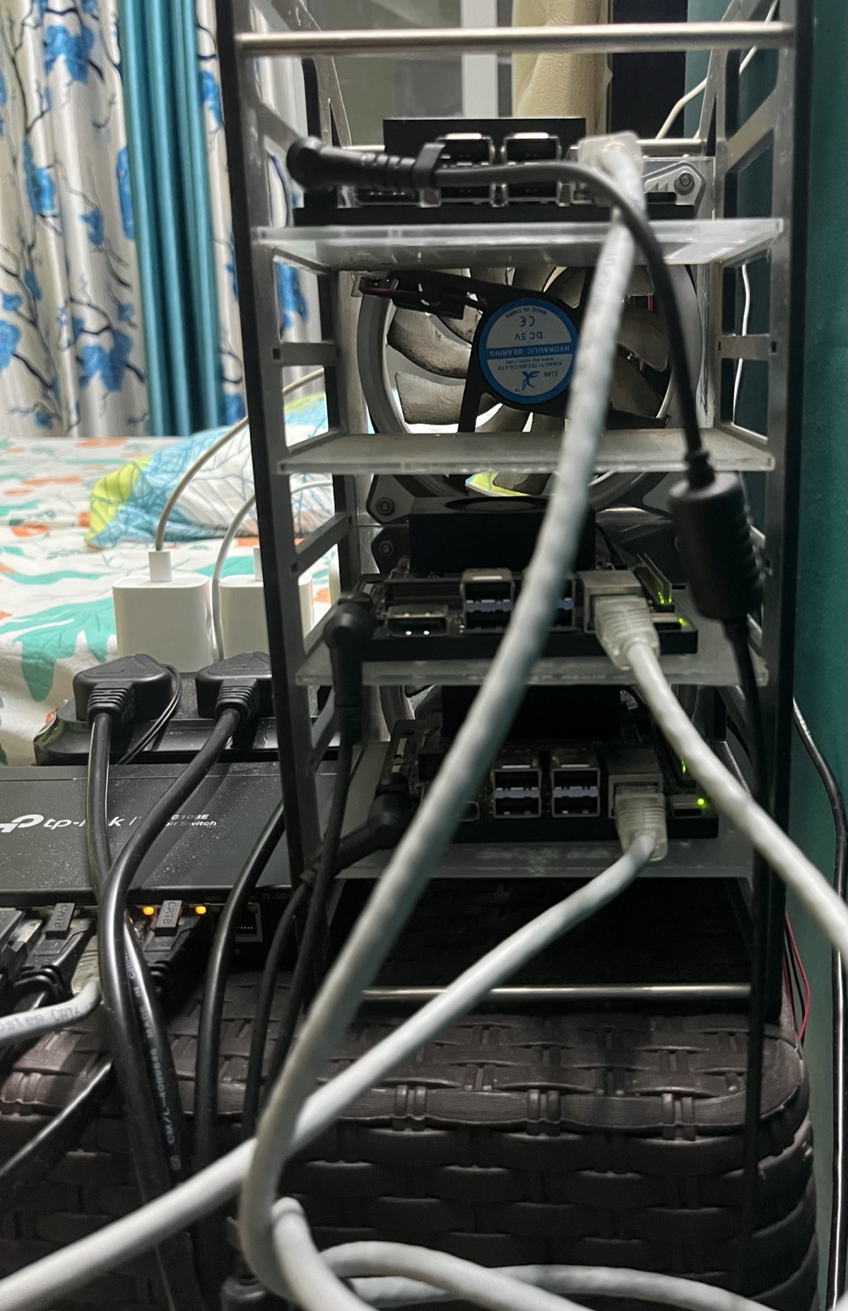 My Jetson Nano Orin Super cluster setup - its real!
Benchmark Configuration
| Platform | NVIDIA Jetson Orin Nano Super 8GB |
| CPU | 6-core Arm Cortex-A78AE |
| GPU | NVIDIA Ampere (1024 CUDA cores, 32 Tensor cores) |
| Memory | 8 GB LPDDR5 shared CPU+GPU |
| JetPack | R36.4.7 (L4T 36.4) |
| Backend | llama.cpp CUDA, -ngl 99 (all layers on GPU), --no-cache-prompt |
| Runs | Four full sweeps: 7W, 15W, 25W, MAXN_SUPER |
| Sweep | prompt ∈ {256, 512, 1024, 2048} tok × gen ∈ {128, 256, 512} tok × 20 reqs/combo |
| Concurrency | 1 (single-user) |
| Key metric | output tok/J |
Github for scripts and code available at link.
Executive Summary
Five Bonsai-family 1-1.53bit LLMs were benchmarked across all four Jetson Orin Nano Super power modes: 7W, 15W, 25W, and MAXN_SUPER. Each model ran 12 combinations of prompt × generation length (20 requests per combo) at every power mode where it could load.
Key finding:
- 25W is the energy-efficiency sweet spot for all models ≤4B parameters. For Bonsai-8B, 15W and 25W deliver near-identical output tok/J (~1 % difference), making 15W the more power-conservative choice.
- MAXN costs 10–11 % more energy per token than 25W across every model tested.** 25W delivers 47–48 % more output tok/s than 15W while maintaining or improving output tok/J for sub-4B models (ctx=2048, gen=512).
- No thermal throttling was observed at any power mode - peak junction temperature (TJ) reached 75.3 °C at MAXN (Bonsai-8B), well below the 95 °C hardware throttle threshold. All other models peak below 72 °C even at MAXN.
Throughput and efficiency winner at each mode (ctx=2048, gen=512, Ternary-Bonsai-1.7B dominates):
Table 1: Throughput and efficiency winner at each power mode
| Mode | Fastest model | Output Tok/s | Output Tok/J |
|---|---|---|---|
| 7W | Ternary-Bonsai-1.7B | 9.0 | 4.64 |
| 15W | Ternary-Bonsai-1.7B | 23.4 | 4.94 |
| 25W | Ternary-Bonsai-1.7B | 34.7 | 5.18 |
| MAXN | Ternary-Bonsai-1.7B | 38.0 | 4.55 |
Ternary-Bonsai-8B (Q2_0, ~1.4 GB) failed at every power mode: OOM in 8 GB unified memory when combined with KV cache and CUDA overhead. All five remaining models have complete data across all four power modes.
Data Availability
Complete per-cell JSON exports (all 33 metrics, all 12 prompt×gen combos × 20 requests per cell) are published on Hugging Face Datasets:
| Mode | Dataset | Models | Cells |
|---|---|---|---|
| 7W | YuvrajSingh9886/bonsai-jetson-benchmark-7w |
5 | 60 |
| 15W | YuvrajSingh9886/bonsai-jetson-benchmark-15w |
5 | 60 |
| 25W | YuvrajSingh9886/bonsai-jetson-benchmark-25w |
5 | 60 |
| MAXN | YuvrajSingh9886/bonsai-jetson-benchmark-maxn |
5 | 60 |
Each dataset contains the full profile_export_aiperf.json per cell (all 33 metrics including ISL, OSL, TTFT avg/p50/p90/p99, ITL, output tok/s, request latency, prefill tok/s, power W, output tok/J), tegrastats.log, and per-model server logs.
1. Test Setup
1.1 Hardware
Table 2: Hardware configuration
| Component | Detail |
|---|---|
| Board | Jetson Orin Nano Super 8GB (Developer Kit) |
| CPU | 6× Arm Cortex-A78AE @ up to 1.728 GHz |
| GPU | NVIDIA Ampere, 1024 CUDA cores, 32 Tensor cores |
| Memory | 8 GB LPDDR5 102 GB/s (unified CPU + GPU) |
| CMA | 256 MB (contiguous memory pool; depletes across sequential model loads) |
| Cooling | Active fan; peak junction temperature ≤ 75 °C across all modes |
1.2 Software Stack
| Layer | Version / Detail |
|---|---|
| OS / JetPack | JetPack R36.4.7 (Ubuntu 22.04, L4T 36.4) |
| CUDA | 12.6 |
| llama.cpp | CUDA backend, -ngl 99, --no-cache-prompt --cache-ram 0 |
| Inference server | llama-server: host 0.0.0.0:8080, --parallel 1, -c 2560 |
| Load generator | aiperf (NVIDIA AI Performance tool) |
| Power telemetry | tegrastats at 500 ms, VDD_CPU_GPU_CV rail (mW) |
| Python | 3.10 (aiperf-env), pandas, seaborn, matplotlib |
| Datasets | Synthetic prompts at exact token counts (256, 512, 1024, 2048) generated synthetically via aiperf |
| Concurrency | 1 user, 1 request at a time (--parallel 1, --concurrency 1) - single-user latency and throughput profile only |
| Batch size | 512 tokens physical (-ub / ubatch, default) · 2048 logical (-b, default) for llama.cpp |
1.3 Models Under Test
| Model | Quant | GGUF size | Tokenizer |
|---|---|---|---|
| Bonsai-1.7B | Q1_0 | ~237 MB | Qwen/Qwen3-1.7B |
| Bonsai-4B | Q1_0 | ~540 MB | Qwen/Qwen3-4B |
| Bonsai-8B | Q1_0 | ~1.1 GB | Qwen/Qwen3-8B |
| Ternary-Bonsai-1.7B | Q2_0 | ~300 MB | Qwen/Qwen3-1.7B |
| Ternary-Bonsai-4B | Q2_0 | ~700 MB | Qwen/Qwen3-4B |
| Ternary-Bonsai-8B | Q2_0 | ~1.4 GB | N/A |
1.4 Power Modes
Table 5: Power mode configurations
| Mode | nvpmodel | GPU clock | CPU clock | VDD_CPU_GPU_CV (observed) |
|---|---|---|---|---|
| 7W | -m 3 |
~408 MHz | 960 MHz | 0.5–2.5 W under load |
| 15W | -m 0 |
~612 MHz | 1 190 MHz | 3–7 W under load |
| 25W | -m 1 |
~820 MHz | 1 420 MHz | 4–10 W under load |
| MAXN | -m 2 + jetson_clocks |
1 020 MHz | 1 728 MHz | 6–12 W under load |
1.5 Benchmark Methodology
- For each
model×prompt×gen combo,aiperfsends 20 single-concurrency requests with synthetic prompts at the exact target token count. - Power is sampled from
tegrastatsVDD_CPU_GPU_CV(mW → W) at 500 ms intervals. Tegrastats samples are assigned to exact prefill/decode phase windows using per-request nanosecond timestamps fromprofile_export.jsonl.output_tok_J=OSL÷ (decode_power_W×decode_time_p50_s) - decode energy only, prefill excluded. See Appendix H.3. - Clocks were locked with
jetson_clocksat all modes. - Each run’s power and clock speed was capped at x W through
nvpmodeland monitored for thermal stability (no sustained throttling;junction temp≤ 75 °C). - Latency percentile used throughout: all
TTFT,ITL, and request latency (RL) values reported in charts, tables, and energy calculations use the p50 (median) over the 20 requests per combo. The mean is not used for latency because occasional slow requests (GC pause, memory compaction, OS scheduling) inflate it without reflecting typical behaviour. p90 and p99 are available in the raw per-mode report files (Data Availability) for tail-latency analysis.
2. Results: Charts
All charts use data from all four power modes.
2.1 Throughput vs Prompt Length
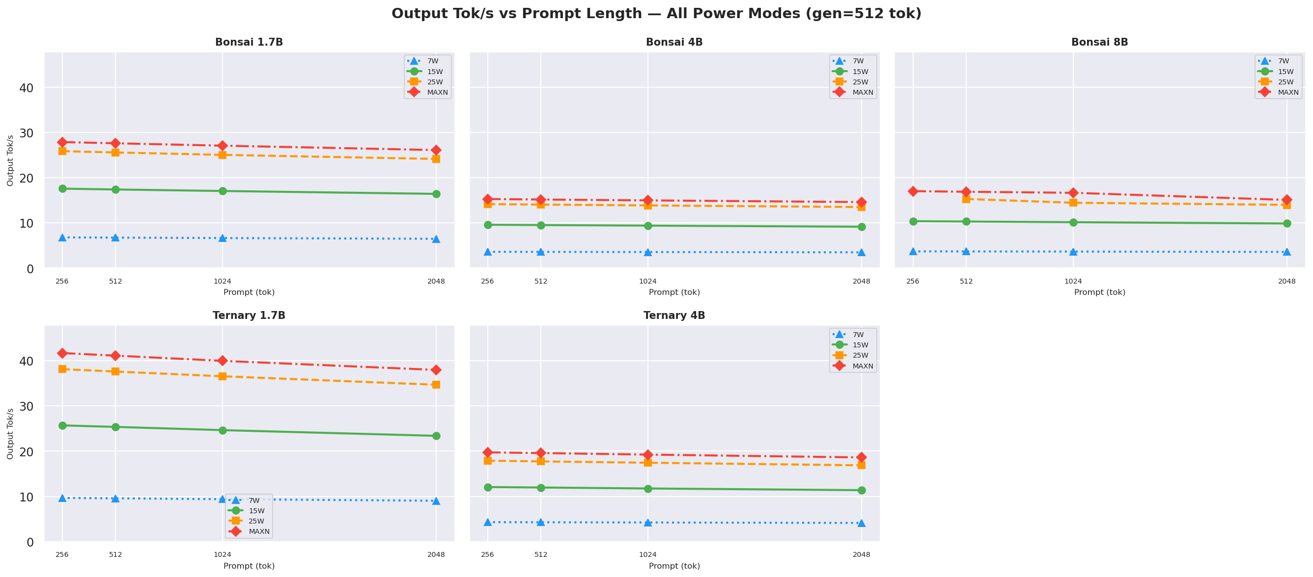
Output tok/s vs prompt length at gen=512 across all models and modes; 25W (orange) consistently leads for models ≤4B:
Figure 1: Output tok/s vs prompt length (gen=512, all models and modes)
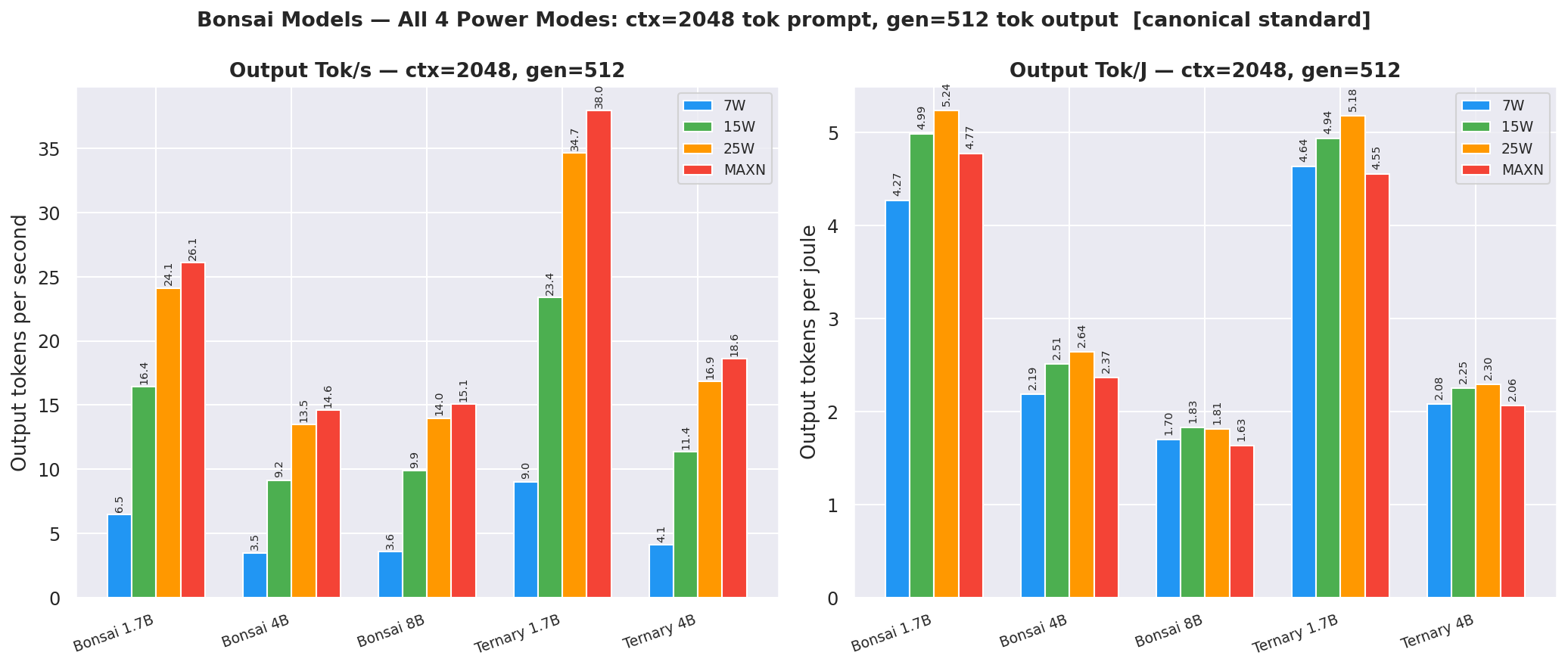
Canonical cell (ctx=2048, gen=512), side-by-side output tok/s and output tok/J bars for all 4 modes:
Figure 2: Canonical cell: output tok/s and tok/J side by side (ctx=2048, gen=512)
2.2 Energy Efficiency
Output Tok/J vs prompt lengthat gen=512; 25W leads for ≤4B models; 15W and 25W are near-tied for Bonsai-8B:
Figure 3: Output tok/J vs prompt length (gen=512, all models and modes)

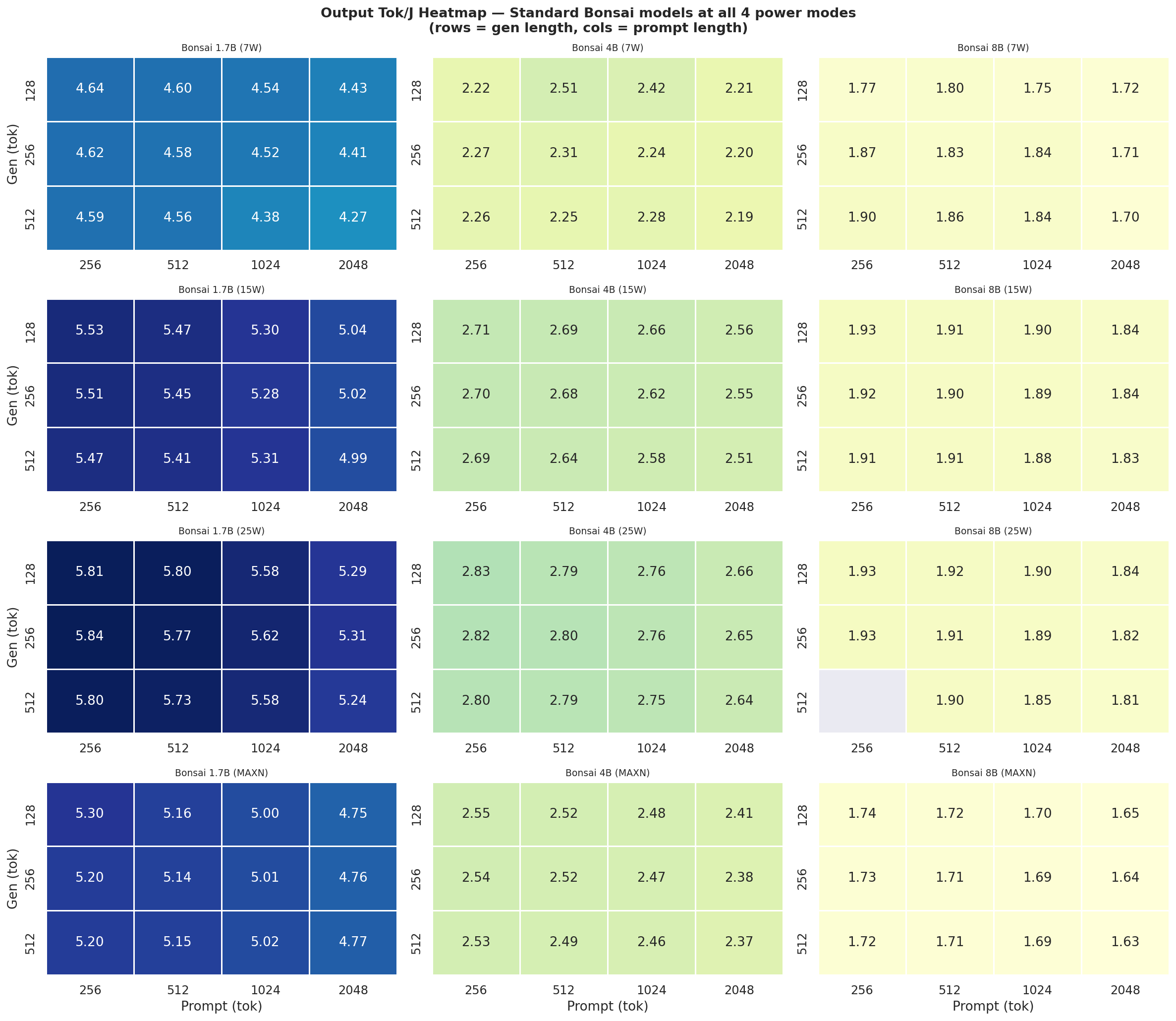
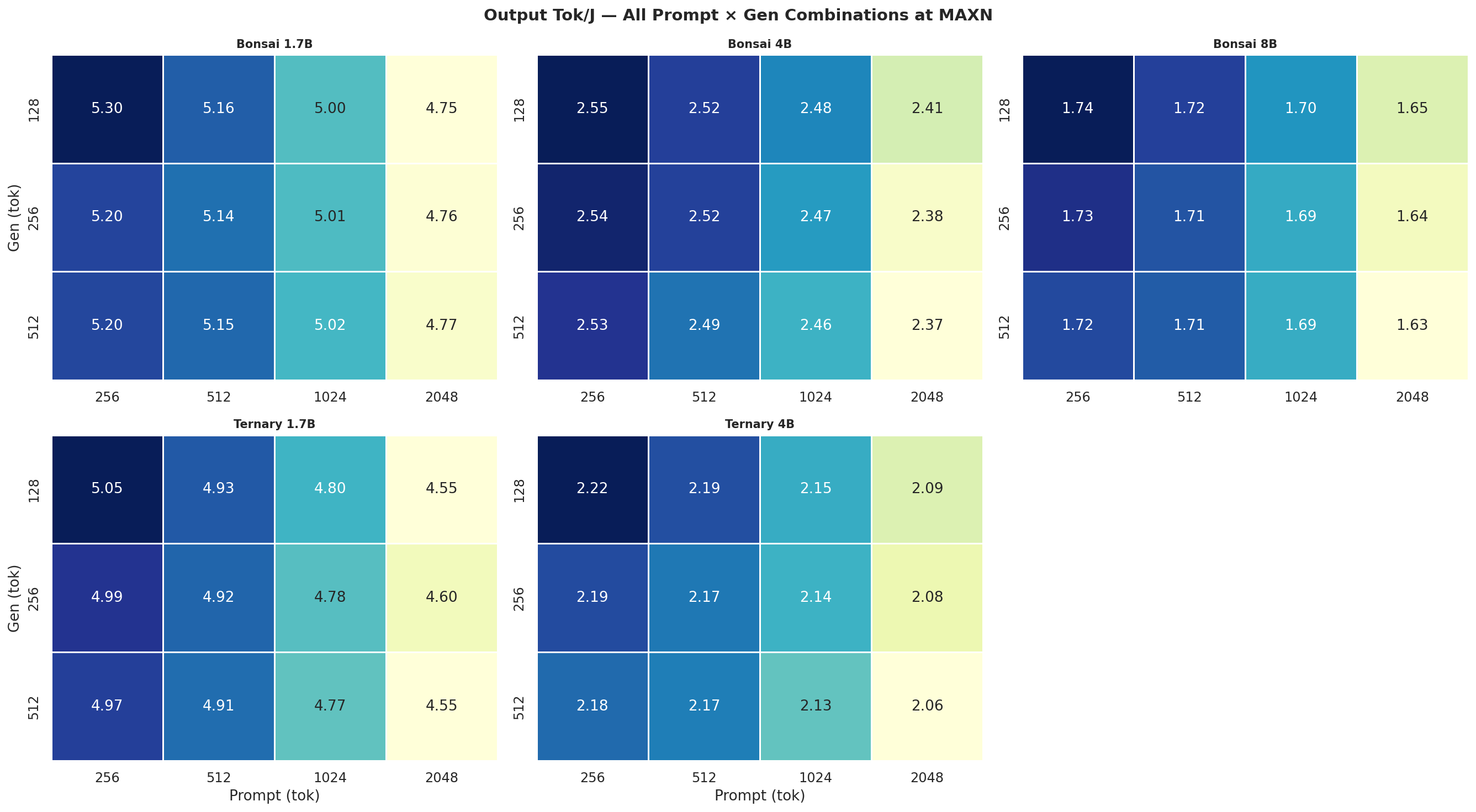
Output Tok/J heatmap(gen × prompt) for Standard Bonsai models (1.7B, 4B, 8B) at all 4 modes:
Figure 4: Output tok/J heatmap: Standard Bonsai models at all 4 power modes (gen × prompt)
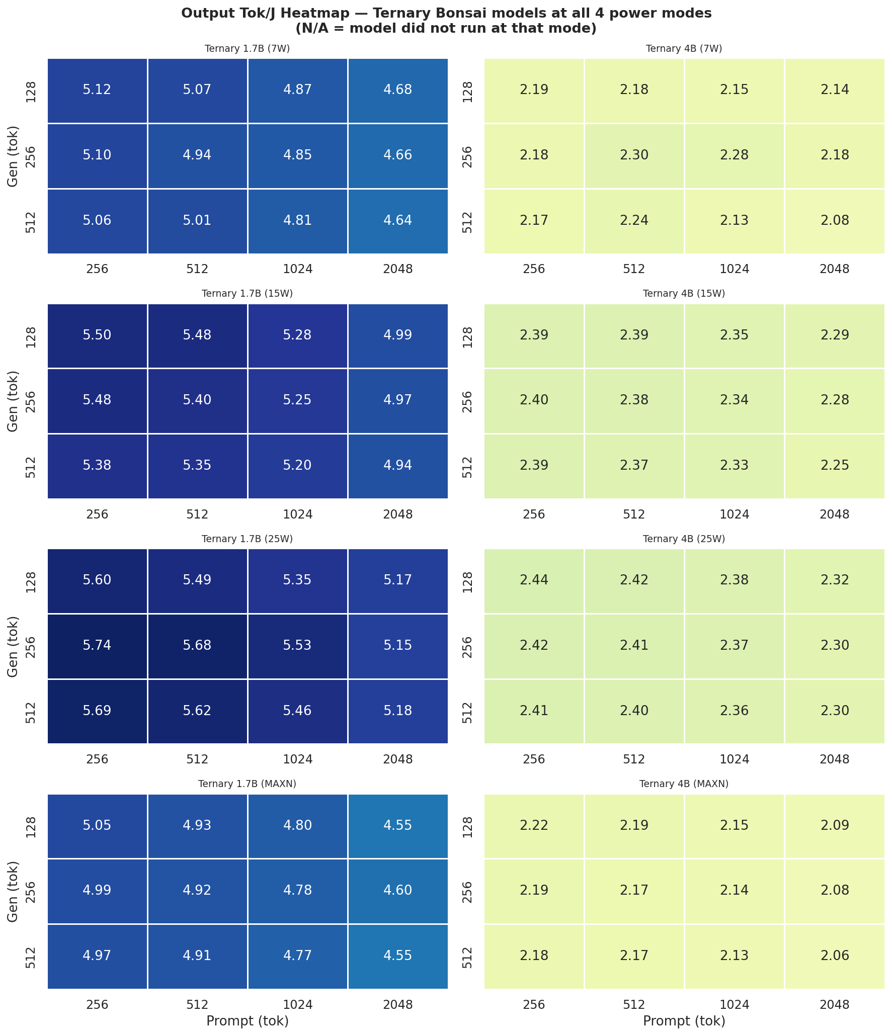
Output Tok/J heatmapfor Ternary Bonsai models (1.7B, 4B) at all 4 power modes:
Figure 5: Output tok/J heatmap: Ternary Bonsai models at all 4 power modes (gen × prompt)
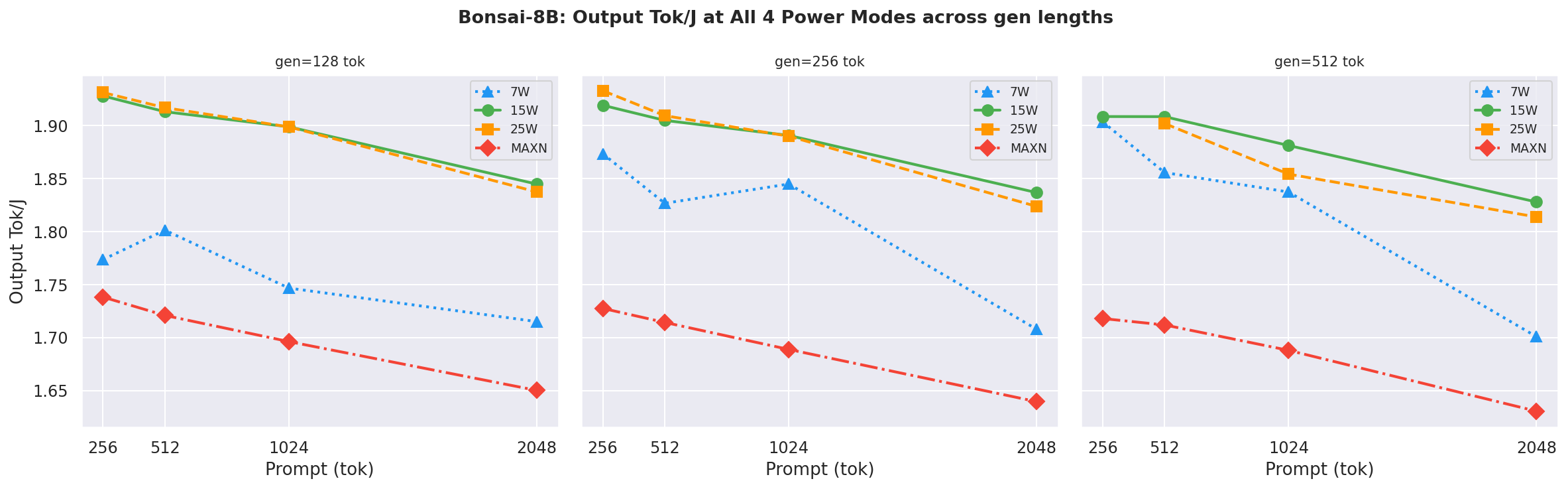
Bonsai-8B spotlight: output tok/J at all 4 power modes across all three gen lengths - the model where 15W and 25W are energy-equivalent:
Figure 6: Bonsai-8B output tok/J at all 4 power modes across gen lengths
Prefill tok/J(input tokens per joule of prefill energy) vs prompt length at gen=512, how efficiently each mode processes the prompt; higher is better:
Figure 7a: Prefill tok/J (input tok / J) vs prompt length (gen=512, all models and modes)
Note:
prefill_tok_J=ISL/ (prefill_power_W×TTFT_s) usesprefill_power_Wderived from tegrastats samples assigned to exact prefill windows using per-request nanosecond timestamps (request_start_ns→request_ack_ns) fromprofile_export.jsonl. Prefill draws significantly more power than decode on Bonsai models (up to ~1.6x for 1.7B/4B). See Appendix H.5 for the full methodology.

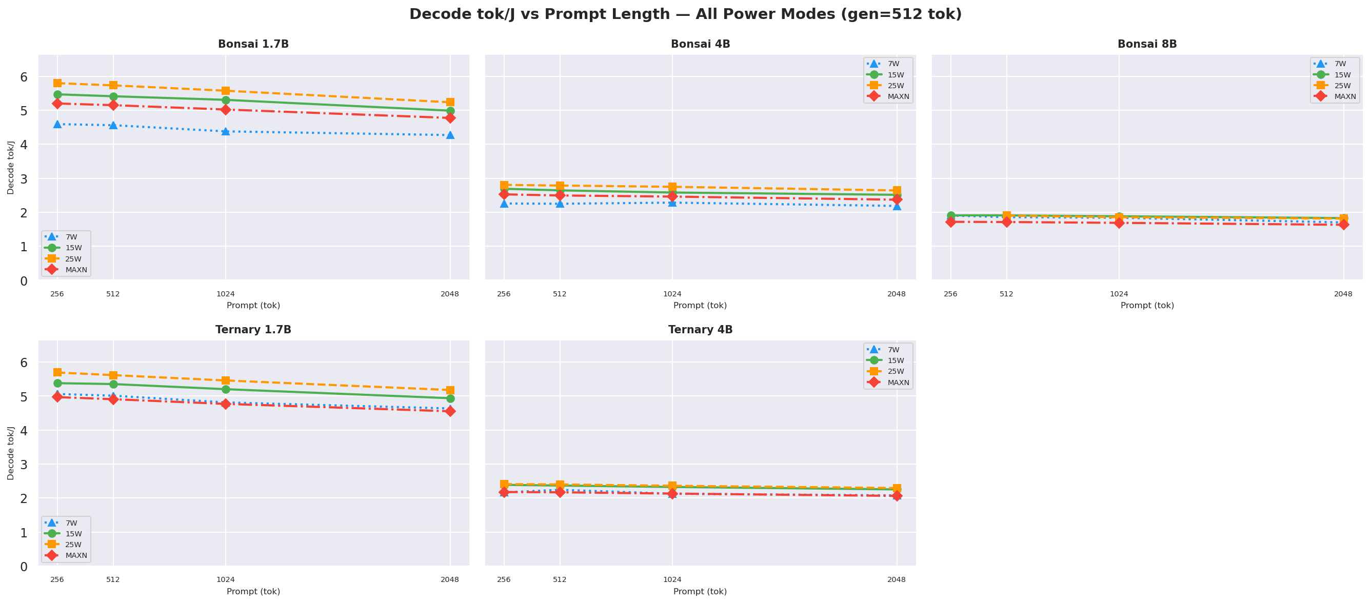
Decode tok/J(output tokens per joule of decode energy) vs prompt length at gen=512, output generation efficiency; 25W leads for sub-4B models:
Figure 7b: Decode tok/J (output tok / J) vs prompt length (gen=512, all models and modes)
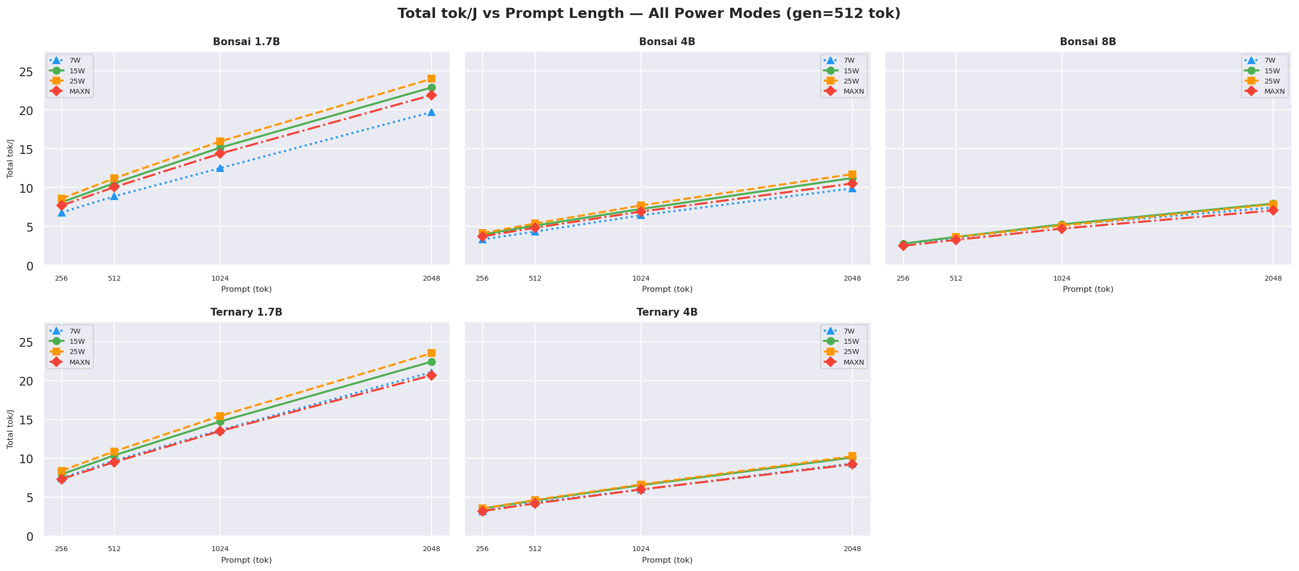
Total tok/J((input + output) tokens per joule of total request energy) vs prompt length at gen=512, overall request efficiency; 25W wins for sub-4B models at every prompt length:
Figure 7c: Total tok/J (input+output tok / J) vs prompt length (gen=512, all models and modes)
Phase power draw at the canonical cell (ctx=2048, gen=512) - the wattage each phase actually draws, showing why prefill and decode have different energy costs:
Figure 7d: Prefill phase power (W) - all models × all power modes (ctx=2048, gen=512)
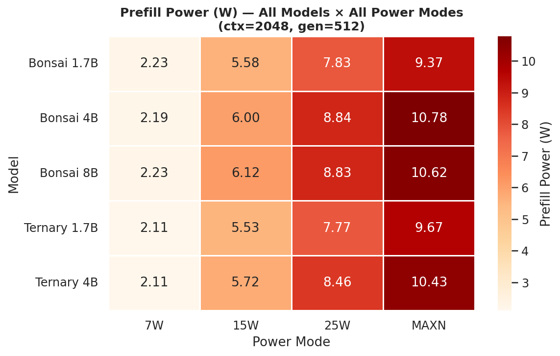
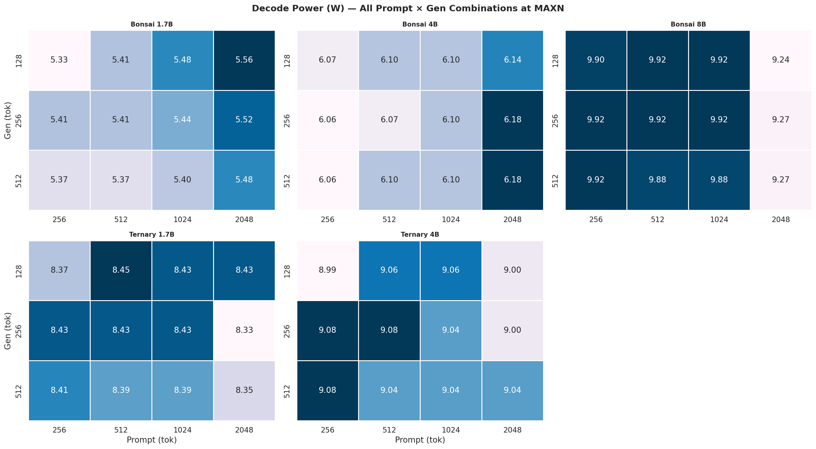
Figure 7e: Decode phase power (W) - all models × all power modes (ctx=2048, gen=512)
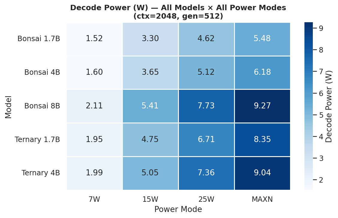
Prefill is a fully-batched forward pass over the prompt (compute-heavy); decode is one token at a time (memory-bandwidth bound). Prefill consistently draws more watts than decode at the same power mode. Per-mode heatmaps across all 12 prompt × gen combinations: C.3 Phase Power.
Full tok/J charts for all ctx/gen combinations: D.1 Prefill · D.2 Decode · D.3 Total.
2.3 Latency
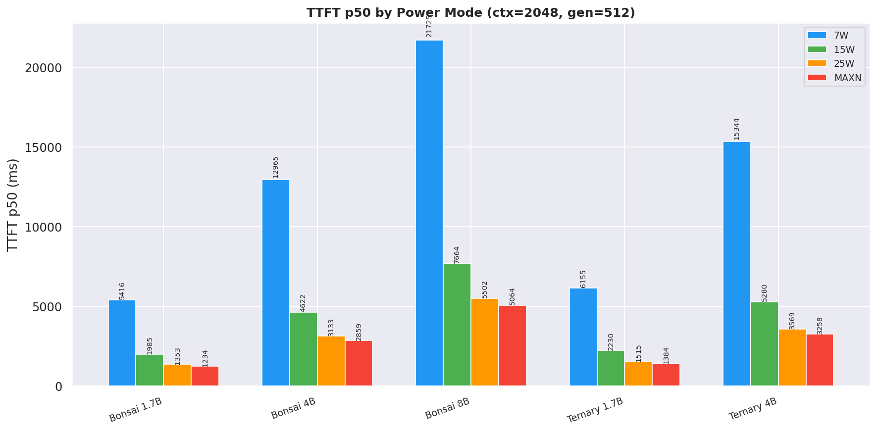
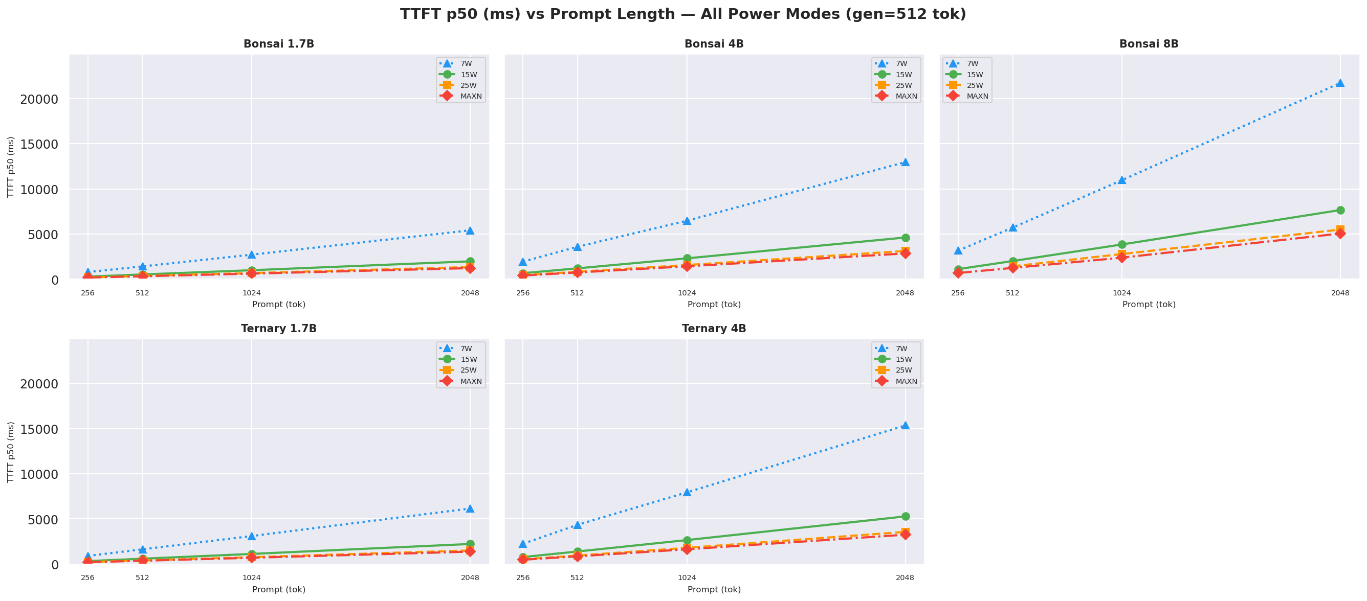
TTFT p50 at ctx=2048, gen=512; 25W and MAXN reduce TTFT by 29–39 % vs 15W:
Figure 8: TTFT p50 by power mode (ctx=2048, gen=512)
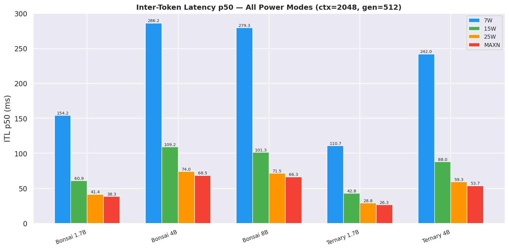
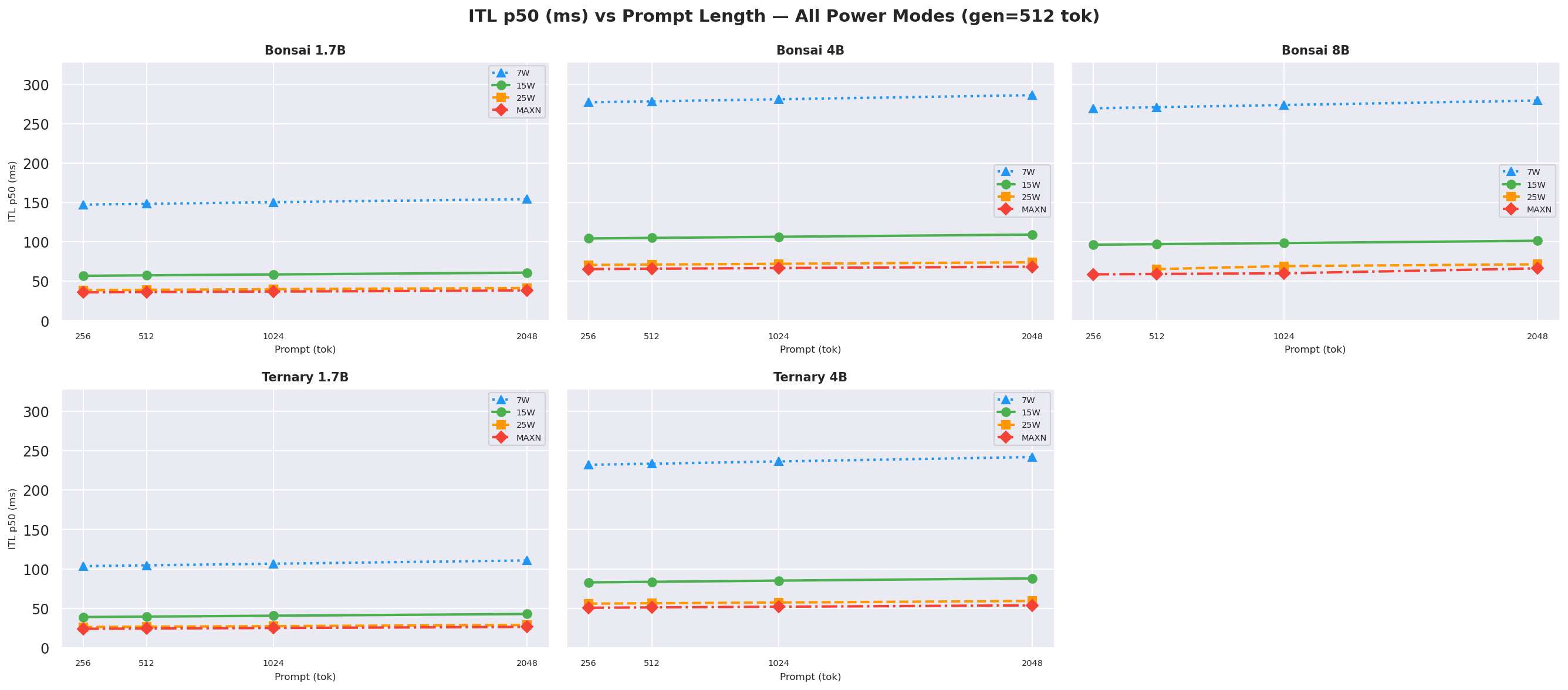
ITL (inter-token latency) p50 at ctx=2048, gen=512; lower is better:
Figure 9: ITL p50 by power mode (ctx=2048, gen=512)
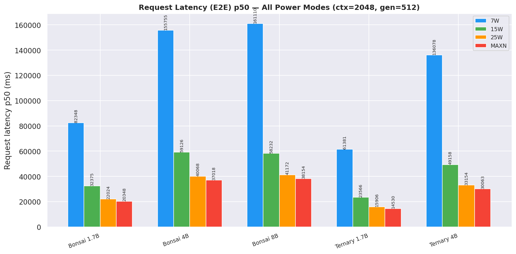
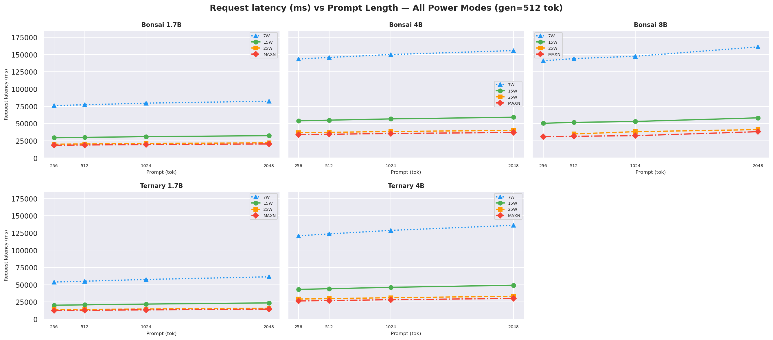
Request latency (E2E) p50 at ctx=2048, gen=512; total time from request start to last token received:
Figure 10: Request latency (E2E) p50 by power mode (ctx=2048, gen=512)
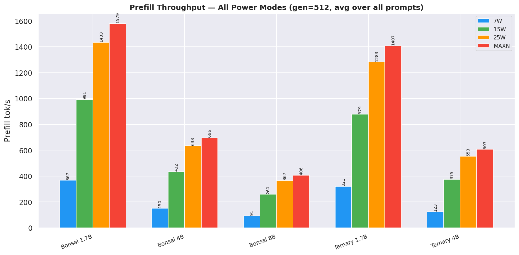
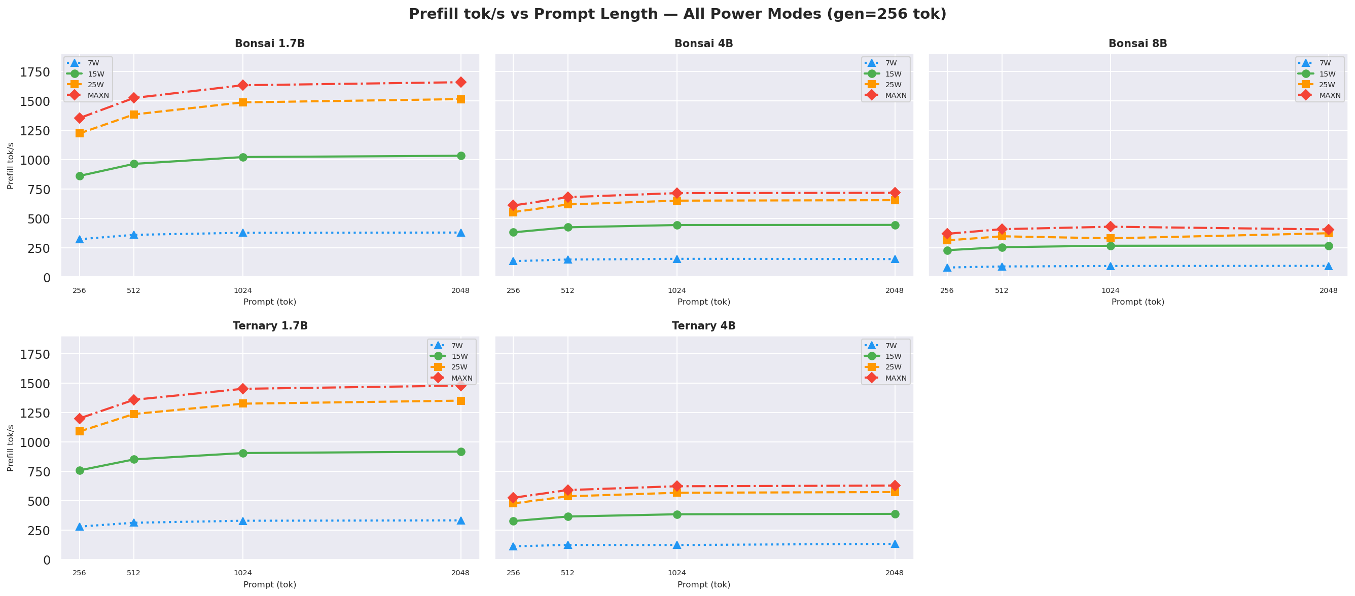
2.4 Prefill Throughput
25W and MAXN provide ~29–47 % faster prefill than 15W:
Figure 11: Prefill throughput by power mode (gen=512, avg over all prompt lengths)
2.5 Power Draw
Figure 12: Median VDD_CPU_GPU_CV power draw per model at each power mode
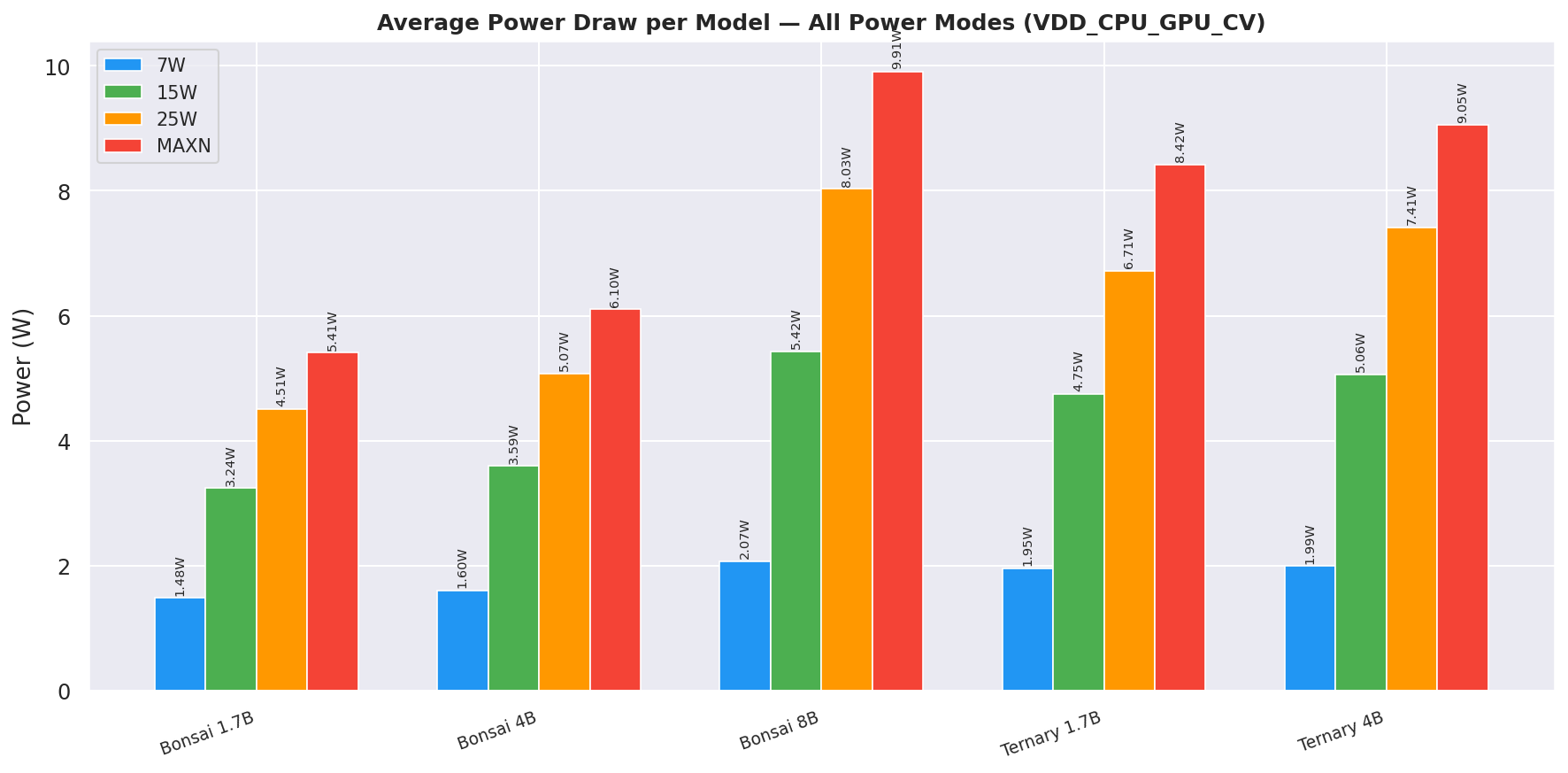
Table 6: Median power draw per model at each power mode (W, VDD_CPU_GPU_CV)
| Model | 7W | 15W | 25W | MAXN |
|---|---|---|---|---|
| Bonsai-1.7B | 1.48 | 3.24 | 4.51 | 5.41 |
| Bonsai-4B | 1.60 | 3.59 | 5.07 | 6.10 |
| Bonsai-8B | 2.07 | 5.42 | 8.03 | 9.91 |
| Ternary-Bonsai-1.7B | 1.95 | 4.75 | 6.71 | 8.42 |
| Ternary-Bonsai-4B | 1.99 | 5.06 | 7.41 | 9.05 |
Median over all 12 prompt × gen combos. Bold = highest observed power draw per model row.
2.5.1 VDD_IN + VDD_CPU_GPU_CV ≠ TDP
The nvpmodel TDP cap (7W/15W/25W/MAXN) applies to the total module draw, measured by the VDD_IN rail. VDD_CPU_GPU_CV is a subset - they’re not additive:
VDD_IN ≈ VDD_CPU_GPU_CV + VDD_SOC + misc rails
-
The wattage looks low as in table 6 because the
VDD_CPU_GPU_CVrail only captures the GPU, CPU, and CV engine power - not the entire module. The remaining power is drawn by other components (memory controller, media blocks, I/O, DRAM self-refresh, PMIC losses) that are outside the scope ofVDD_CPU_GPU_CVbut still contribute to the total power budget under the TDP cap. -
Since, we only test single-user, single-request mode, there isn’t enough load to push the total module power up to the TDP ceiling.
VDD_IN               ≈ 7.5W  (total module - well under the 15W cap)
├── VDD_CPU_GPU_CV    = 3.2W  (CPU + GPU + CV engine)
├── VDD_SOC           = 1.7W  (memory controller, media blocks)
└── other rails       ≈ 2.6W  (misc I/O, DRAM self-refresh, PMIC losses)
No thermal throttling was triggered at any mode because the Bonsai decode workload never saturates the GPU compute units - the TDP ceiling is never approached.
3. Analysis
3.1 Higher tok/sec != efficient model (tok/J)
Tok/s (left half) and tok/J (right half) are intentionally both shown- a faster mode does not always mean a more efficient one.
- MAXN beats 25W on raw tok/s (+8–11 %) for all models but loses on tok/J (−10–11 %) because its power increase outpaces the throughput gain for ctx = 2048, gen = 512.
output_tok_J=OSL/ (decode_power_W×decode_time_p50_s) - decode energy only. See Appendix H.3 for full formula.
Full breakdown across all 12 ctx × gen combinations: Appendix I.
Table 7: Canonical cell comparison (ctx=2048, gen=512)
| Model | 7W tok/s | 15W tok/s | 25W tok/s | MAXN tok/s | 7W tok/J | 15W tok/J | 25W tok/J | MAXN tok/J | Peak tok/J |
|---|---|---|---|---|---|---|---|---|---|
| Bonsai-1.7B | 6.5 | 16.4 | 24.1 | 26.1 | 4.27 | 4.99 | 5.24 | 4.77 | 25W |
| Bonsai-4B | 3.5 | 9.2 | 13.5 | 14.6 | 2.19 | 2.51 | 2.64 | 2.37 | 25W |
| Bonsai-8B | 3.6 | 9.9 | 14.0 | 15.1 | 1.70 | 1.83 | 1.81 | 1.63 | 15W |
| Ternary-Bonsai-1.7B | 9.0 | 23.4 | 34.7 | 38.0 | 4.64 | 4.94 | 5.18 | 4.55 | 25W |
| Ternary-Bonsai-4B | 4.1 | 11.4 | 16.9 | 18.6 | 2.08 | 2.25 | 2.30 | 2.06 | 25W |
3.2 The 25W Sweet Spot
25W is the best mode for output tok/J and tok/sec for all sub-4B Bonsai models, and is near-parity for Bonsai-8B. The arithmetic is:
- Going from 15W → 25W: output tok/s rises 47–48 % (GPU clock 612 → 820 MHz), while power rises ~38–46 %. Net output tok/J gain: +1 to +6 % for 1.7B–4B models (including Ternary-Bonsai-4B: 2.25 → 2.30); −1 % for Bonsai-8B (memory-bandwidth bound, clock gain wiped by power overhead).
- Going from 25W → MAXN: output tok/s gains +8–11 % (decode is memory-bandwidth bound, not compute bound), while power rises ~20–25 %. Net output tok/J loss: −10 to −11 % across all models.
The GPU clock ceiling at 15W (612 MHz) leaves significant decode throughput on the table for sub-8B models. Raising it to 820 MHz at 25W captures most of the available improvement at modest extra power. The final jump to 1020 MHz at MAXN costs disproportionate power for marginal gains.
3.3 Best use cases for each power mode
Table 8: Recommended power mode by use case
| Use case | Recommended mode |
|---|---|
| Always-on inference (sub-4B) | 25W: best output tok/J and tok/sec balance; vs 15W: +47-48% tok/s, +46-48% TTFT, +2-5% output tok/J |
| Interactive chat, real-time response (sub-4B) | MAXN: lowest prefill time (TTFT) and highest tok/sec; vs 25W: +8-10% tok/s, +10% prefill time (TTFT), -9-12% output tok/J |
| Power-constrained / thermally limited (sub-4B) | 15W: saves 28-32% power vs 25W; vs 25W: -32% tok/s, -32% TTFT, -2-5% output tok/J |
| Edge AI / Smartphone deployment | 7W: all 8 models fit (reboot per run required); vs 15W: -61-64% tok/s, -63-68% TTFT, -6-14% output tok/J; lowest power budget |
All above numbers are for sub-4B models tested. For 8B models performance, please check the individual sections for your interest.
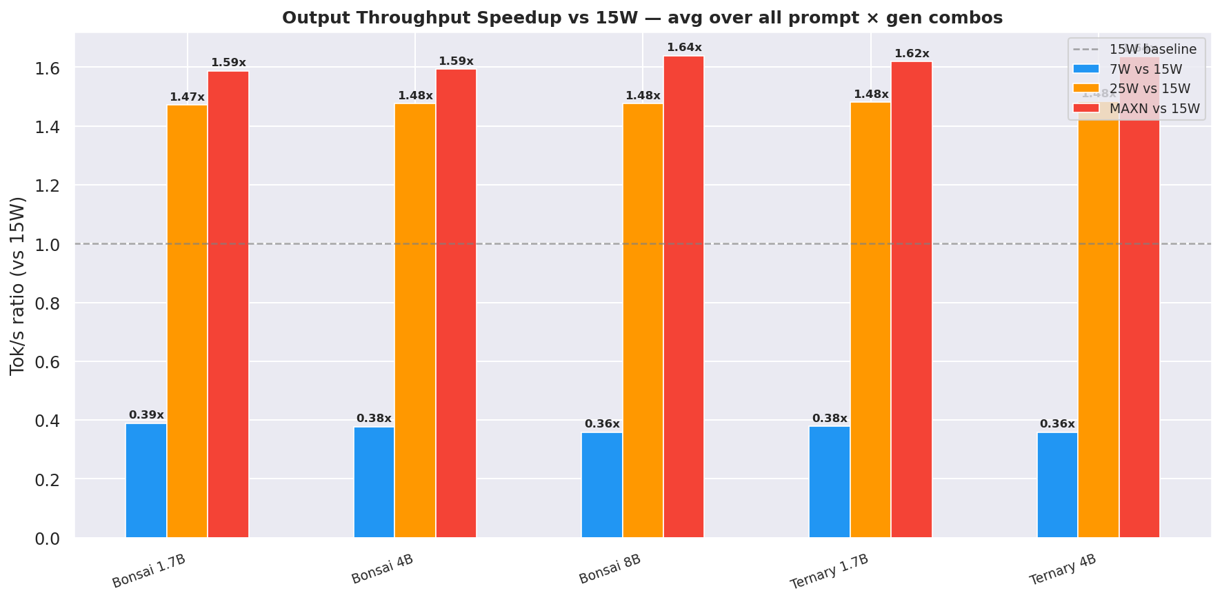
3.4 Throughput Speedup Summary
All figures are median(p50) across the full prompt × gen sweep (12 combos per model); throughput uses median(p50 tok/s).
Table 9: Output throughput speedup ratios - all pairwise mode comparisons
| Model | 25W / 15W | MAXN / 15W | 15W / 7W | 25W / 7W | MAXN / 7W | MAXN / 25W |
|---|---|---|---|---|---|---|
| Bonsai-1.7B | 1.47x | 1.59x | 2.57x | 3.78x | 4.08x | 1.08x |
| Bonsai-4B | 1.48x | 1.59x | 2.65x | 3.90x | 4.22x | 1.08x |
| Bonsai-8B | 1.48x | 1.64x | 2.79x | 4.11x | 4.57x | 1.11x |
| Ternary-Bonsai-1.7B | 1.48x | 1.62x | 2.64x | 3.92x | 4.28x | 1.09x |
| Ternary-Bonsai-4B | 1.48x | 1.64x | 2.79x | 4.13x | 4.56x | 1.10x |
- 25W delivers a consistent ~1.47–1.48x speedup vs 15W across all models.
- 15W gives about 2.5–2.8x boost vs 7W; Bonsai-8B and Ternary-4B show the largest gain at 2.78x.
- MAXN/25W is consistently ~1.08–1.10x for all models - extra compute headroom over an already-fast 25W baseline translates to only modest gains, since decode is memory-bandwidth bound.
- MAXN/7W reaches 4.56x for Ternary-Bonsai-4B - the largest speedup in the sweep. 25W/7W for Ternary-Bonsai-4B is 4.13x, the highest 25W gain of any model.
- For Bonsai models (1.4B/4B), the throughput is consistenly higher compared to Ternary models.
Figure 14: Output throughput speedup vs 15W baseline - all models and modes
3.5 Latency Characteristics
TTFT scales near-linearly with prompt across all modes. At ctx=256 a model like Bonsai-1.7B prefills in ~170 ms (25W); at ctx=2048 that grows to ~1353 ms.
Inter-token latency (ITL) p50 is the median per-token decode cost. ITL heatmaps per power mode (all 5 models, all 12 prompt×gen combos) are in Appendix F.2 - see Figures F.2a–F.2d. At the canonical ctx=2048, gen=512:
7W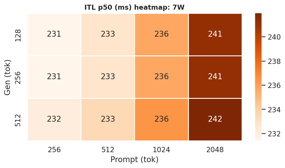 |
15W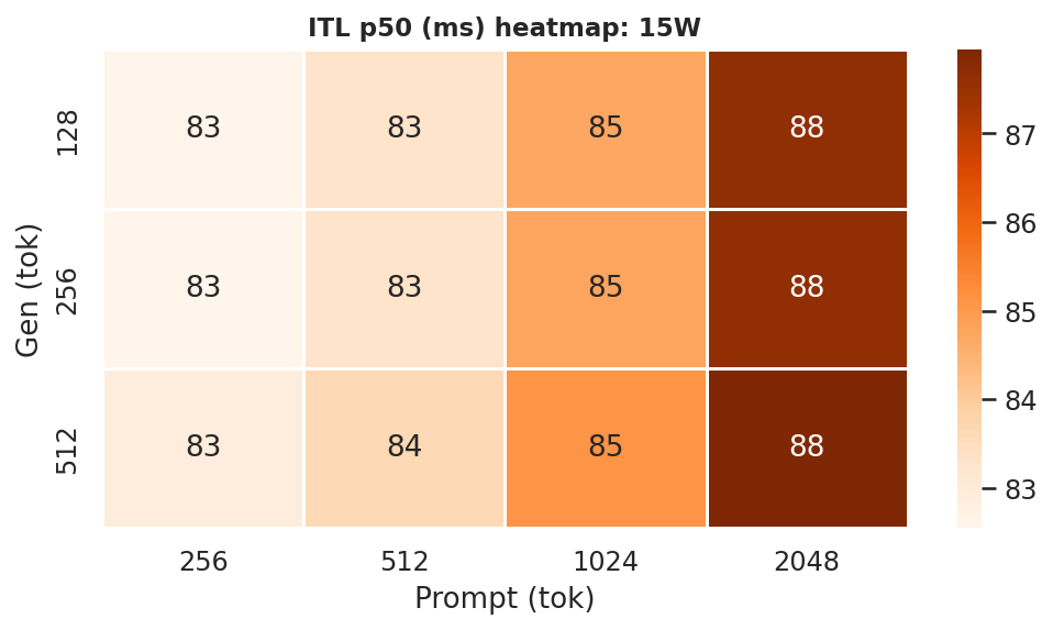 |
25W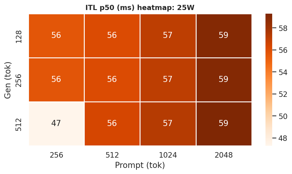 |
MAXN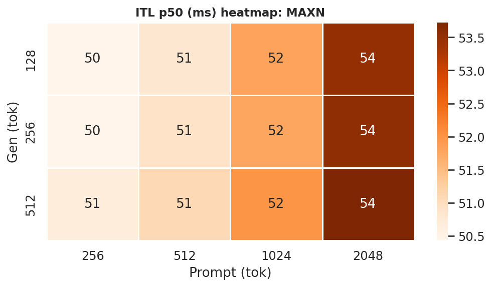 |
Figure 10a: ITL p50 heatmaps - all 4 power modes (rows = gen length, cols = prompt length)
ITLis driven primarily by model size and GPU clock (or power mode) but also loosely on prompt length too, like between ctx length=256 to ctx length=2048, theITLincreases because of the larger context (prompt + generation -> kv cache scans increases too). Bonsai models have lowerITLthan Ternary models at every mode.- The Ternary-Bonsai-1.7B achieves lower
ITLthan Bonsai-1.7B at every mode despite larger file size, consistent with ternary weights being faster to load from DRAM per decode step.
Decode time (s) p50 is the time spent generating output tokens.
Table 10a: Decode time speedup ratios - all pairwise mode comparisons
| Model | 25W vs 15W | MAXN vs 15W | 15W vs 7W | 25W vs 7W | MAXN vs 7W | MAXN vs 25W |
|---|---|---|---|---|---|---|
| Bonsai-1.7B | 1.47x | 1.58x | 2.57x | 3.78x | 4.08x | 1.08x |
| Bonsai-4B | 1.48x | 1.59x | 2.65x | 3.91x | 4.22x | 1.08x |
| Bonsai-8B | 1.50x | 1.64x | 2.79x | 4.17x | 4.57x | 1.10x |
| Ternary-Bonsai-1.7B | 1.48x | 1.62x | 2.64x | 3.92x | 4.28x | 1.09x |
| Ternary-Bonsai-4B | 1.48x | 1.64x | 2.79x | 4.13x | 4.56x | 1.10x |
See Appendix H.9 for the full speedup formula. decode_time =
RLp50 −TTFTp50; median over all 12 prompt × gen combos.
- Decode time for Ternary models is lower than those of Bonsai models. Why?
- The reason lies in 1-bit vs 1.58-bit model structure. Bonsai’s 1-bit quantization requires more complex bit unpacking and on-the-fly dequantization during decode, which adds overhead per token. Ternary’s 2-bit structure with optimized ternary-CUDA kernels allows for more efficient memory access patterns and simpler decode logic, reducing per-token latency despite the larger file size.
Thinking with Claude, there is this amusing reason, since 1.58-bits (-1,0,1} has ‘0’ as a valid weight, it can skip the multiply-accumulate for those zero weights during dequant stage (conversion to fp16 or bf16 for GEMM), while 1-bit quantization has to do the full compute for every weight bit, even if many are effectively zero after unpacking. This leads to more efficient decoding for the ternary models.
TTFT speedup - median(TTFT_baseline) / median(TTFT_mode) over all 12 prompt × gen combos (see H.9):
Table 11: TTFT speedup ratios - all pairwise mode comparisons
| Model | 25W vs 15W | MAXN vs 15W | 15W vs 7W | 25W vs 7W | MAXN vs 7W | MAXN vs 25W |
|---|---|---|---|---|---|---|
| Bonsai-1.7B | 1.46x | 1.60x | 2.71x | 3.95x | 4.34x | 1.10x |
| Bonsai-4B | 1.47x | 1.61x | 2.86x | 4.21x | 4.62x | 1.10x |
| Bonsai-8B | 1.29x | 1.56x | 2.84x | 3.66x | 4.42x | 1.21x |
| Ternary-Bonsai-1.7B | 1.46x | 1.60x | 2.75x | 4.02x | 4.41x | 1.10x |
| Ternary-Bonsai-4B | 1.48x | 1.62x | 3.08x | 4.54x | 4.98x | 1.10x |
- Bonsai-8B shows a smaller
TTFTimprovement at 25W vs 15W (1.29x) compared to the 4B models (1.47–1.48x). This confirms the prefill is also becoming memory-bandwidth bound for the larger model. - MAXN/7W reaches 4.98x for Ternary-Bonsai-4B prefill - the largest
TTFTspeedup in the sweep. 25W/7W is 4.54x for Ternary-Bonsai-4B, also the highest across all models at that comparison.
Request latency (E2E) speedup - median(RL p50 at baseline) / median(RL p50 at mode) over all 12 prompt × gen combos (see H.9):
Table 12: Request latency (E2E) speedup ratios - all pairwise mode comparisons
| Model | 25W vs 15W | MAXN vs 15W | 15W vs 7W | 25W vs 7W | MAXN vs 7W | MAXN vs 25W |
|---|---|---|---|---|---|---|
| Bonsai-1.7B | 1.47x | 1.59x | 2.57x | 3.78x | 4.09x | 1.08x |
| Bonsai-4B | 1.47x | 1.60x | 2.66x | 3.92x | 4.24x | 1.08x |
| Bonsai-8B | 1.51x | 1.60x | 2.79x | 4.21x | 4.47x | 1.06x |
| Ternary-Bonsai-1.7B | 1.48x | 1.62x | 2.64x | 3.91x | 4.28x | 1.09x |
| Ternary-Bonsai-4B | 1.48x | 1.64x | 2.81x | 4.16x | 4.59x | 1.10x |
- Mirrors the
TTFTspeedup trends since prefill dominates request latency at these context sizes.
3.6 Model Size vs Efficiency
The relationship is clear: smaller quantized models always win on total tok/J, not just tok/s.
Table 13: Best total tok/J ranked by model size
| Model | Params | GGUF | Best total tok/J | At mode / ctx / gen |
|---|---|---|---|---|
| Bonsai-1.7B | 1.7B | ~237 MB | 62.5 | 25W / 2048 / 128 |
| Ternary-Bonsai-1.7B | 1.7B | ~300 MB | 59.6 | 25W / 2048 / 128 |
| Bonsai-4B | 4B | ~540 MB | 28.7 | 25W / 2048 / 128 |
| Ternary-Bonsai-4B | 4B | ~700 MB | 25.5 | 25W / 2048 / 128 |
| Bonsai-8B | 8B | ~1.1 GB | 18.8 | 15W / 2048 / 128 |
Total tok/J = (
ISL+OSL) / (p50_power_W×RL_p50_s) - see Appendix H.6 for the full formula. Peaks at ctx=2048, gen=128 for every model because the long prompt dominates the numerator while short gen minimises decode energy. All 48 mode × ctx × gen combinations were searched.
Figure 13: Best output tok/J per model - all power modes
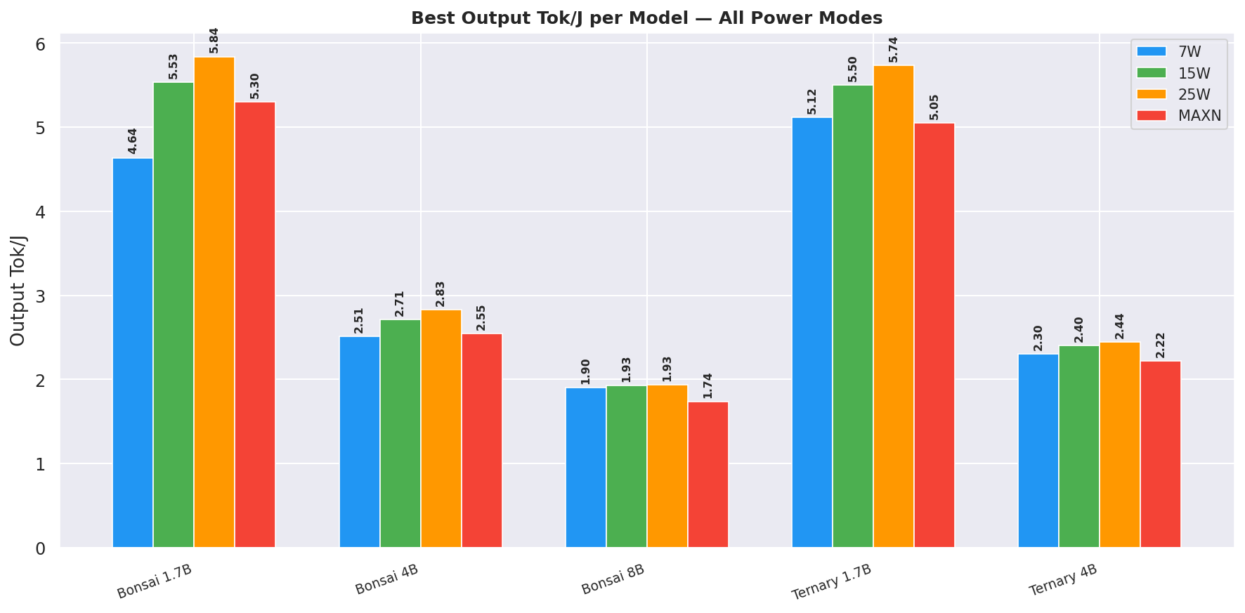
Bonsai-1.7B at 25W achieves 62.5 total tok/J, more than 3× more efficient than Bonsai-8B (18.8) across the full request.
Notably, Bonsai-1.7B edges Ternary-Bonsai-1.7B on total tok/J (62.5 vs 59.6) despite having fewer parameters - the Q1_0 Bonsai-1.7B is slightly lighter on memory bandwidth than the Q2_0 ternary variant. Ternary-Bonsai-1.7B wins on output tok/s and output tok/J at the canonical cell instead.
3.7 Energy Efficiency: Decode tok/J and Total tok/J
Table 14: Request energy split – prefill vs decode % of total request energy (median over all 12 prompt x gen combos)
| Model | Phase | 7W | 15W | 25W | MAXN |
|---|---|---|---|---|---|
| Bonsai-1.7B | Prefill | 7% | 7% | 6% | 6% |
| Bonsai-1.7B | Decode | 93% | 93% | 94% | 94% |
| Bonsai-4B | Prefill | 9% | 9% | 9% | 9% |
| Bonsai-4B | Decode | 91% | 91% | 91% | 91% |
| Bonsai-8B | Prefill | 11% | 12% | 15% | 12% |
| Bonsai-8B | Decode | 89% | 88% | 85% | 88% |
| Ternary-Bonsai-1.7B | Prefill | 9% | 9% | 9% | 9% |
| Ternary-Bonsai-1.7B | Decode | 91% | 91% | 91% | 91% |
| Ternary-Bonsai-4B | Prefill | 10% | 10% | 10% | 10% |
| Ternary-Bonsai-4B | Decode | 90% | 90% | 90% | 90% |
prefill_J=prefill_power_WxTTFT_p50_s;decode_J=decode_power_Wxdecode_time_p50_s;prefill%=prefill_J/ (prefill_J+decode_J). Phase power from tegrastats samples assigned to exact phase windows via per-request nanosecond timestamps. See H.5.
Two complementary tok/J lenses on energy efficiency - see H.6 for formulas:
See Figure 7b (decode tok/J vs prompt length) and Figure 7c (total tok/J vs prompt length) in section 2.2. Full combinations: D.2 Decode · D.3 Total.
Key findings:
-
25W wins on both metrics for sub-4B models at every prompt and gen length. The exception is Bonsai-8B, where 15W and 25W are almost the same on tok/J (1.81 vs 1.83 output tok/J at canonical cell).
-
The 1.7B models reach ~5 tok/J (decode) vs ~2.5–2.7 tok/J for the 4B models and ~1.8 tok/J for Bonsai-8B. Smaller models are dramatically more energy-efficient per output token.
-
Decode dominates request energy. As clearly visible in Table 14, the decode phase accounts for ~90–94 % of total request energy across all models and modes. Prefill is a smaller fraction. The reason is the amount of time spent. Prefill is a one-time cost at the start of the request, while decode is an ongoing cost that accumulates with every generated token. Even though prefill power can be similar to decode power, the much longer duration of decode means it contributes more to total energy.
-
The ternary 1.7B model has slightly lower decode tok/J than Bonsai-1.7B (standard) despite higher raw throughput - the Q2_0 format requires more DRAM bandwidth per token than Q1_0, which slightly increases decode energy relative to throughput.
-
Ternary-Bonsai models draw 10–20 % more decode power than same-size Bonsai-1bit despite both dequantizing to fp16 GEMM. The difference is fully explained by memory bandwidth - not compute intensity:
| Bonsai Q1_0 (1.125 bpw) | Ternary-Bonsai Q2_0 (2.06 bpw) | |
|---|---|---|
| Model size (4B) | 540 MiB | 1,020 MiB |
| Bits per weight | 1.125 | 2.06 |
| Dequant op | sign × scale (trivial) |
2-bit lookup → {-1,0,+1} × scale |
| Bytes read per token | 540 MiB | 1,020 MiB (1.9× more) |
| Power impact | baseline | +10–20 % (DRAM traffic dominates) |
Neither format runs natively on GPU hardware - Q1_0 and Q2_0 both dequantize to fp16 before GEMM. The power gap comes from 1.9× more weight bytes moved through the memory controller in the Ternary variant, not from a difference in compute.
Phase power by mode (W) – median over all 12 prompt × gen combos:
| Model | Phase | 7W | 15W | 25W | MAXN |
|---|---|---|---|---|---|
| Bonsai-1.7B | Prefill | 2.07 | 4.52 | 5.81 | 7.30 |
| Bonsai-1.7B | Decode | 1.48 | 3.22 | 4.50 | 5.41 |
| Bonsai-4B | Prefill | 2.15 | 5.44 | 7.70 | 9.09 |
| Bonsai-4B | Decode | 1.60 | 3.59 | 5.05 | 6.10 |
| Bonsai-8B | Prefill | 2.13 | 5.97 | 8.47 | 10.56 |
| Bonsai-8B | Decode | 2.05 | 5.41 | 8.03 | 9.91 |
| Ternary-Bonsai-1.7B | Prefill | 2.05 | 5.04 | 7.08 | 8.80 |
| Ternary-Bonsai-1.7B | Decode | 1.95 | 4.75 | 6.71 | 8.42 |
| Ternary-Bonsai-4B | Prefill | 2.05 | 5.49 | 7.90 | 9.62 |
| Ternary-Bonsai-4B | Decode | 1.99 | 5.06 | 7.41 | 9.04 |
Table 14a: Prefill power ratios – all pairwise mode comparisons
| Model | 25W/15W | MAXN/15W | 15W/7W | 25W/7W | MAXN/7W | MAXN/25W |
|---|---|---|---|---|---|---|
| Bonsai-1.7B | 1.29x | 1.62x | 2.18x | 2.80x | 3.52x | 1.26x |
| Bonsai-4B | 1.42x | 1.67x | 2.53x | 3.57x | 4.22x | 1.18x |
| Bonsai-8B | 1.42x | 1.77x | 2.80x | 3.97x | 4.95x | 1.25x |
| Ternary-Bonsai-1.7B | 1.40x | 1.75x | 2.46x | 3.45x | 4.29x | 1.24x |
| Ternary-Bonsai-4B | 1.44x | 1.75x | 2.68x | 3.85x | 4.69x | 1.22x |
Table 14b: Decode power ratios – all pairwise mode comparisons
| Model | 25W/15W | MAXN/15W | 15W/7W | 25W/7W | MAXN/7W | MAXN/25W |
|---|---|---|---|---|---|---|
| Bonsai-1.7B | 1.40x | 1.68x | 2.17x | 3.04x | 3.65x | 1.20x |
| Bonsai-4B | 1.41x | 1.70x | 2.25x | 3.16x | 3.81x | 1.21x |
| Bonsai-8B | 1.48x | 1.83x | 2.64x | 3.91x | 4.83x | 1.23x |
| Ternary-Bonsai-1.7B | 1.41x | 1.77x | 2.43x | 3.44x | 4.31x | 1.25x |
| Ternary-Bonsai-4B | 1.46x | 1.79x | 2.54x | 3.72x | 4.54x | 1.22x |
Ratios show how much more power mode A draws vs mode B (ratio > 1 = A draws more). Computed from
VDD_CPU_GPU_CVtegrastats samples assigned to prefill/decode phase windows via per-request nanosecond timestamps; median over all 12 prompt x gen combos. See H.5 for phase assignment methodology.
Key observations:
- Prefill draws more power than decode at every mode for sub-4B models (prefill is compute-bound; decode is memory-bandwidth-bound). Bonsai-8B is the exception – its decode power approaches prefill at higher modes because of higher FLOPS and memory bandwidth demands and so does the energy too.
- 25W vs 15W adds only 1.29-1.48x power but delivers 1.47-1.50x throughput – the sweet spot where each extra watt of draw returns more than proportional speed.
- MAXN vs 25W adds just 1.18-1.26x power on prefill and 1.20-1.25x on decode, yet delivers only +8-10% tok/s (1.08-1.10x) and loses -9-12% output tok/J – the diminishing-returns zone where the power increase outpaces the out tok/sec and tok/J gain because of single-user, single-request setup not able to fully utilzie the extra GPU headroom.
- 7W decode power (1.48-2.05 W) is remarkably low – the SoC at minimum clocks draws less than a typical USB charger during autoregressive generation.
Figure 15: Total energy per request vs output length at 25W, ctx=2048
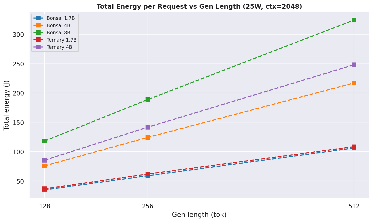
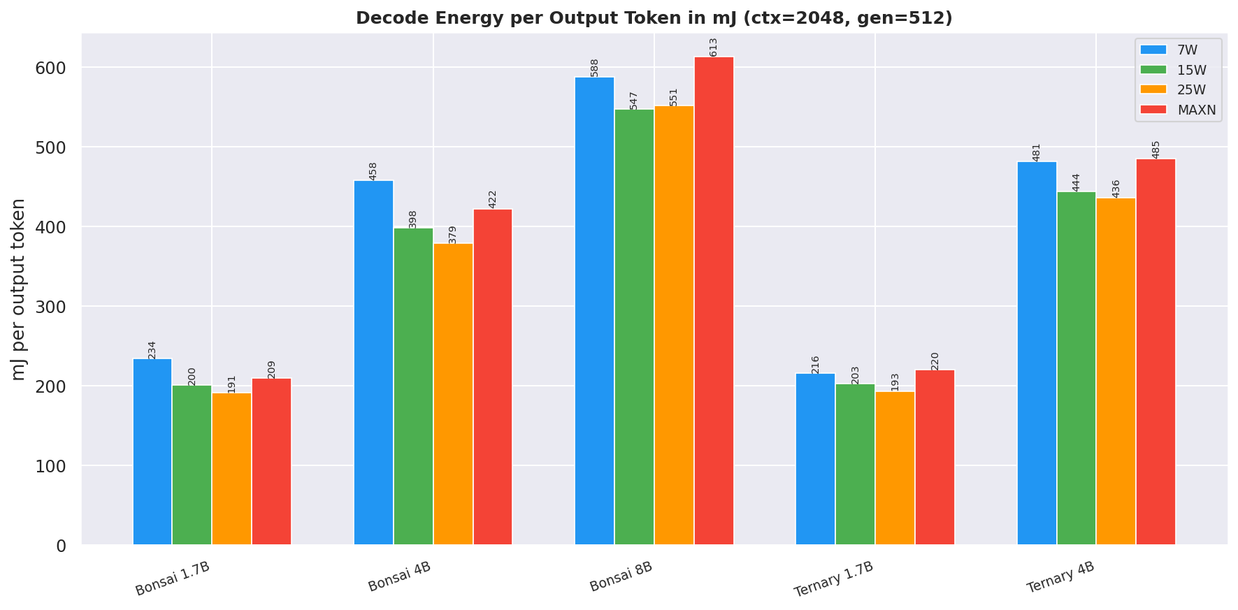
Figure 16: Decode energy per output token in mJ (ctx=2048, gen=512)
4. Conclusion
What These Numbers Mean for Edge Inference
At Ternary-Bonsai-1.7B Q2_0:
- up to 38.4 tok/s at 25W (ctx=256): real-time fluent generation
- 0.24 s
TTFTat ctx=256 (25W) - ~300 MB on disk: trivially portable
- 6.83 W under load: runs on a USB-C power bank
- 5.74 output tok/J (ctx=256, gen=256): best output tok/J for the Ternary-1.7B at 25W
Bonsai-1.7B Q1_0 pushes even further: 5.84 output tok/J (ctx=256, gen=256) in only 237 MB at 4.51 W average under load, 26.0 tok/s and 0.21 s TTFT (25W, ctx=256). Total tok/J peaks at 62.5 (ctx=2048, gen=128, best in suite) where the long prompt dominates the numerator.
- The standard Q1_0 models are lighter on disk and memory bandwidth; the Ternary Q2_0 variants generate faster output tokens per second, thus Ternary models are better for latency-sensitive applications while Bonsai models are mostly energy-efficient per output token.
The Clear Winner: 25W Mode (for sub-4B models)
25W (nvpmodel -m 1) is the Pareto-optimal power mode for Bonsai-1.7B and Bonsai-4B inference on the Jetson Orin Nano Super. It is the right answer for the majority of deployments:
- ~47 % more throughput than 15W (1.7B class) and ~46-47 % faster
TTFT(prefill time) - Only ~40 % more power than 15W
- 10–11 % better output tok/J than MAXN (25W: 2.30–5.24 output tok/J across sub-4B models at ctx=2048, gen=512; up to 5.84 at ctx=256)
- Low peak power (≤ 7 W for 1.7B–4B models) for sustained operation; peak TJ 65.9-66.2 °C – over 28 °C of thermal headroom before the 95 °C hardware throttle threshold
For Bonsai-8B: prefer 15W for energy-efficiency-neutral operation at ~43 % lower board power than 25W.
Appendix A: Full 4-Mode Comparison (ctx=2048, gen=512)
Raw numbers from the canonical benchmark cell. All latencies in milliseconds. Power =
VDD_CPU_GPU_CVmedian over each run window.
Table 15: Full 4-mode comparison, ctx=2048, gen=512
| Model | Mode | Output Tok/s | TTFT p50 (ms) |
ITL p50 (ms) |
Power (W) | Output Tok/J |
|---|---|---|---|---|---|---|
| Bonsai-1.7B | 7W | 6.5 | 5416.1 | 154.18 | 1.52 | 4.27 |
| Bonsai-1.7B | 15W | 16.4 | 1985.3 | 60.92 | 3.30 | 4.99 |
| Bonsai-1.7B | 25W | 24.1 | 1353.1 | 41.43 | 4.62 | 5.24 |
| Bonsai-1.7B | MAXN | 26.1 | 1234.5 | 38.31 | 5.52 | 4.77 |
| Bonsai-4B | 7W | 3.5 | 12964.7 | 286.15 | 1.60 | 2.19 |
| Bonsai-4B | 15W | 9.2 | 4622.3 | 109.23 | 3.65 | 2.51 |
| Bonsai-4B | 25W | 13.5 | 3133.3 | 74.04 | 5.12 | 2.64 |
| Bonsai-4B | MAXN | 14.6 | 2858.6 | 68.46 | 6.18 | 2.37 |
| Bonsai-8B | 7W | 3.6 | 21725.1 | 279.33 | 2.11 | 1.70 |
| Bonsai-8B | 15W | 9.9 | 7663.9 | 101.34 | 5.41 | 1.83 |
| Bonsai-8B | 25W | 14.0 | 5502.4 | 71.48 | 7.73 | 1.81 |
| Bonsai-8B | MAXN | 15.1 | 5064.1 | 66.31 | 9.27 | 1.63 |
| Ternary-Bonsai-1.7B | 7W | 9.0 | 6155.3 | 110.67 | 1.95 | 4.64 |
| Ternary-Bonsai-1.7B | 15W | 23.4 | 2229.7 | 42.76 | 4.75 | 4.94 |
| Ternary-Bonsai-1.7B | 25W | 34.7 | 1515.4 | 28.84 | 6.71 | 5.18 |
| Ternary-Bonsai-1.7B | MAXN | 38.0 | 1384.2 | 26.35 | 8.39 | 4.55 |
| Ternary-Bonsai-4B | 7W | 4.1 | 15343.5 | 241.95 | 1.99 | 2.08 |
| Ternary-Bonsai-4B | 15W | 11.4 | 5280.1 | 87.95 | 5.05 | 2.25 |
| Ternary-Bonsai-4B | 25W | 16.9 | 3569.0 | 59.29 | 7.36 | 2.30 |
| Ternary-Bonsai-4B | MAXN | 18.6 | 3257.6 | 53.72 | 9.04 | 2.06 |
| Ternary-Bonsai-8B | all | OOM: too large for 8 GB unified memory at any power mode |
Appendix B: Thermal Summary - All Power Modes
Power and temperature: median over each model’s full benchmark window (all 12 prompt×gen combos). No model triggered thermal throttling at any power mode (threshold ≈ 95 °C).
Junction temperature (TJ) is the hottest internal die temperature on the Jetson SoC, reported by
tegrastatsastj@. It is the primary metric for thermal safety: if TJ reaches ~95 °C, the hardware automatically throttles clocks to prevent damage. Peak TJ < 76 °C across all runs means thermal headroom is ample.
Table 16: Thermal summary - all power modes
| Model | Mode | Avg Power (W) | Avg CPU (°C) | Avg GPU (°C) | Peak TJ (°C) | Throttled |
|---|---|---|---|---|---|---|
| Bonsai-1.7B | 7W | 1.48 | 53.6 | 54.9 | 55.8 | No |
| Bonsai-1.7B | 15W | 3.24 | 55.6 | 56.8 | 59.0 | No |
| Bonsai-1.7B | 25W | 4.51 | 62.5 | 63.7 | 65.9 | No |
| Bonsai-1.7B | MAXN | 5.41 | 62.1 | 63.3 | 65.9 | No |
| Bonsai-4B | 7W | 1.60 | 53.7 | 55.0 | 57.3 | No |
| Bonsai-4B | 15W | 3.59 | 58.3 | 59.5 | 61.7 | No |
| Bonsai-4B | 25W | 5.07 | 62.4 | 63.8 | 66.2 | No |
| Bonsai-4B | MAXN | 6.10 | 63.4 | 64.7 | 67.7 | No |
| Bonsai-8B | 7W | 2.07 | 54.7 | 56.1 | 58.3 | No |
| Bonsai-8B | 15W | 5.42 | 61.1 | 62.5 | 64.6 | No |
| Bonsai-8B | 25W | 8.03 | 66.3 | 67.9 | 70.4 | No |
| Bonsai-8B | MAXN | 9.91 | 69.9 | 71.8 | 75.3 | No |
| Ternary-Bonsai-1.7B | 7W | 1.95 | 54.8 | 56.2 | 57.0 | No |
| Ternary-Bonsai-1.7B | 15W | 4.75 | 61.2 | 62.5 | 63.8 | No |
| Ternary-Bonsai-1.7B | 25W | 6.71 | 64.3 | 65.9 | 69.2 | No |
| Ternary-Bonsai-1.7B | MAXN | 8.42 | 68.2 | 69.7 | 72.4 | No |
| Ternary-Bonsai-4B | 7W | 1.99 | 54.7 | 56.0 | 57.8 | No |
| Ternary-Bonsai-4B | 15W | 5.06 | 60.6 | 62.0 | 63.7 | No |
| Ternary-Bonsai-4B | 25W | 7.41 | 65.7 | 67.2 | 69.3 | No |
| Ternary-Bonsai-4B | MAXN | 9.05 | 68.4 | 70.0 | 71.8 | No |
Appendix C: Full 12-Combination Heatmaps (All Power Modes)
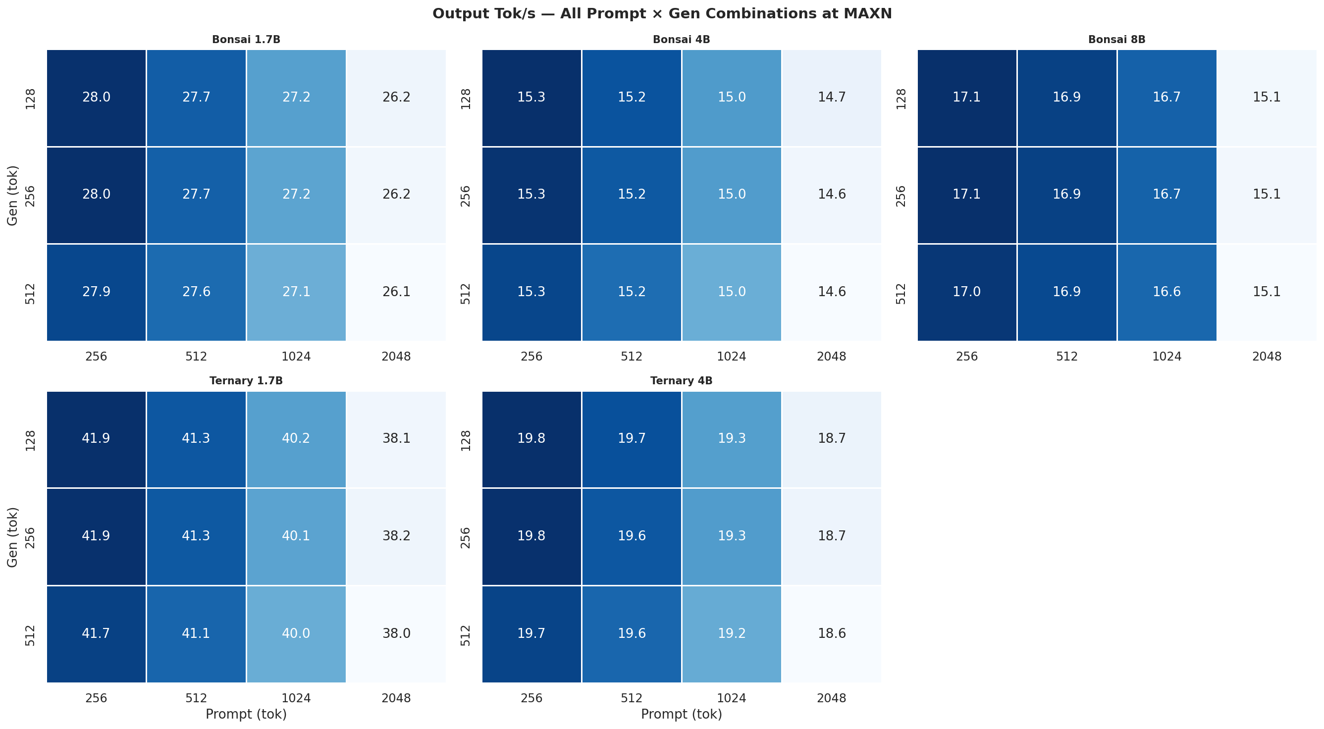
Each heatmap is a 2×3 grid (5 models, 6th panel unused) showing all 12 prompt×gen combinations for one power mode and one metric. Rows = gen length (128, 256, 512 tok), columns = prompt length (256, 512, 1024, 2048 tok). Brighter colour = higher value.
C.1 Output Tok/s heatmaps
Figure C.1a: All 12 combos at 7W
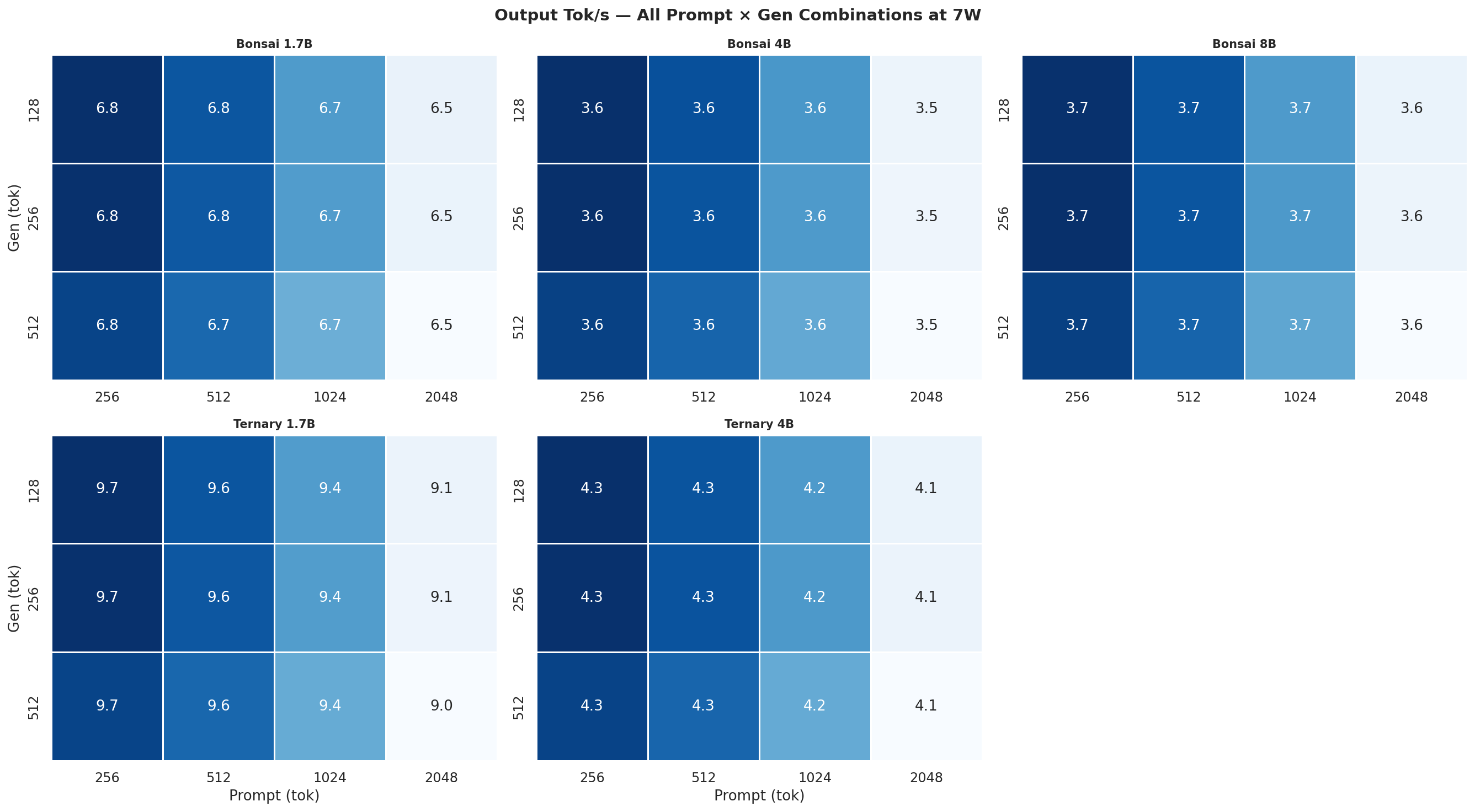
Figure C.1b: All 12 combos at 15W
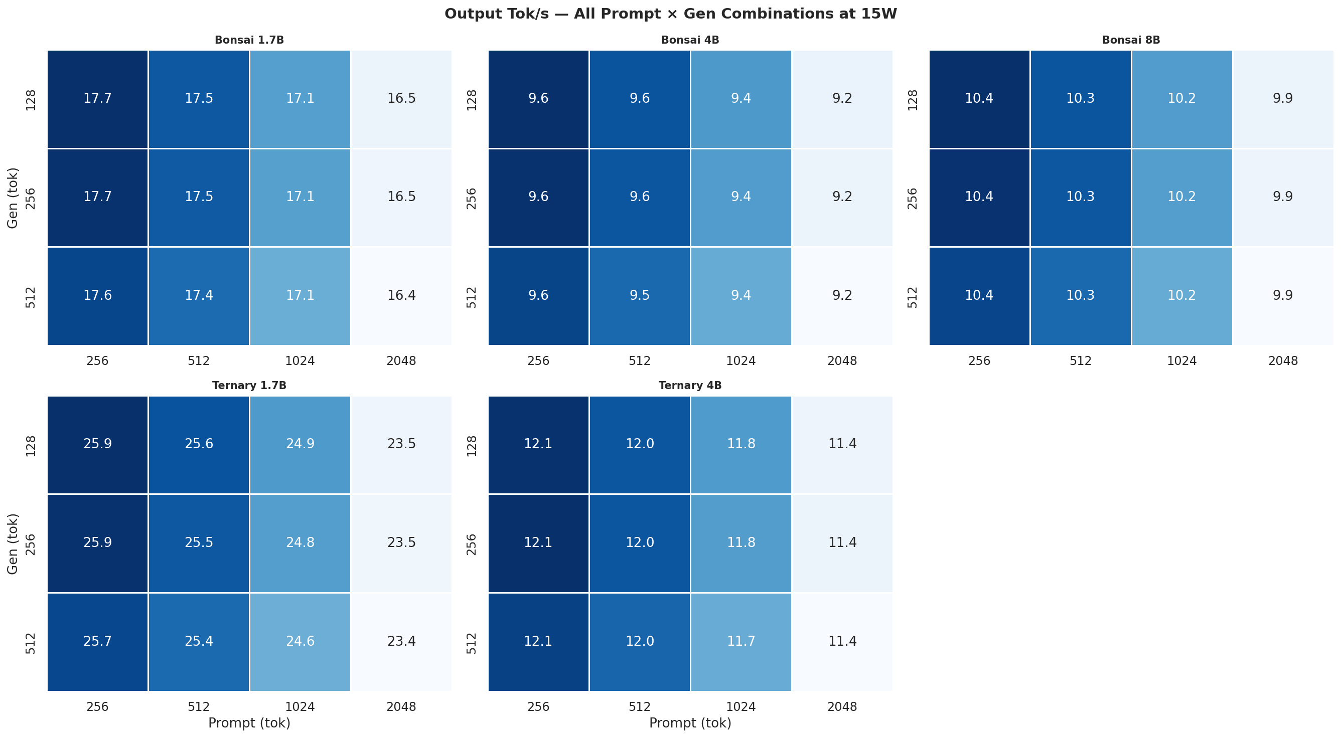
Figure C.1c: All 12 combos at 25W
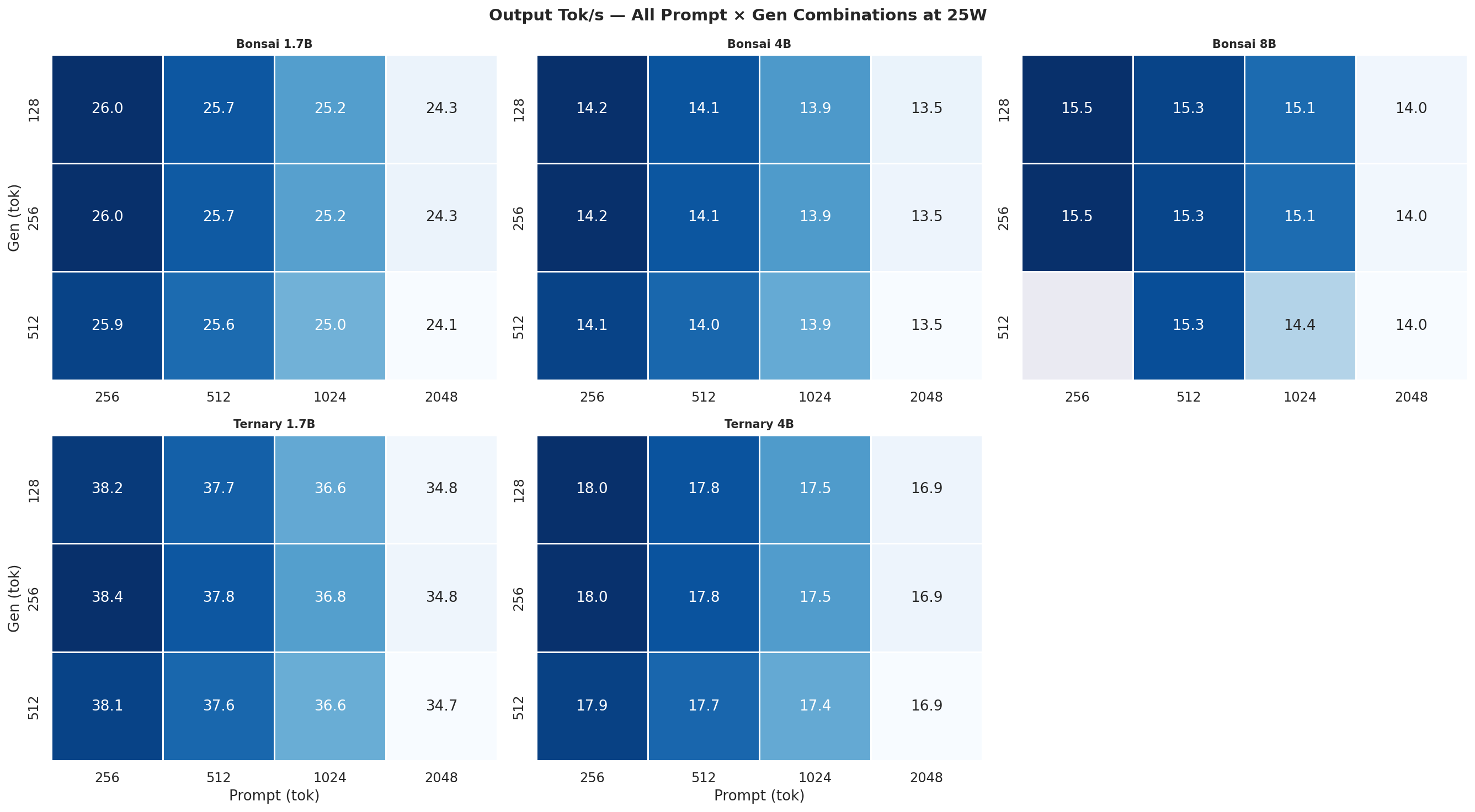
Figure C.1d: All 12 combos at MAXN
C.2 Output Tok/J heatmaps
Figure C.2a: All 12 combos at 7W
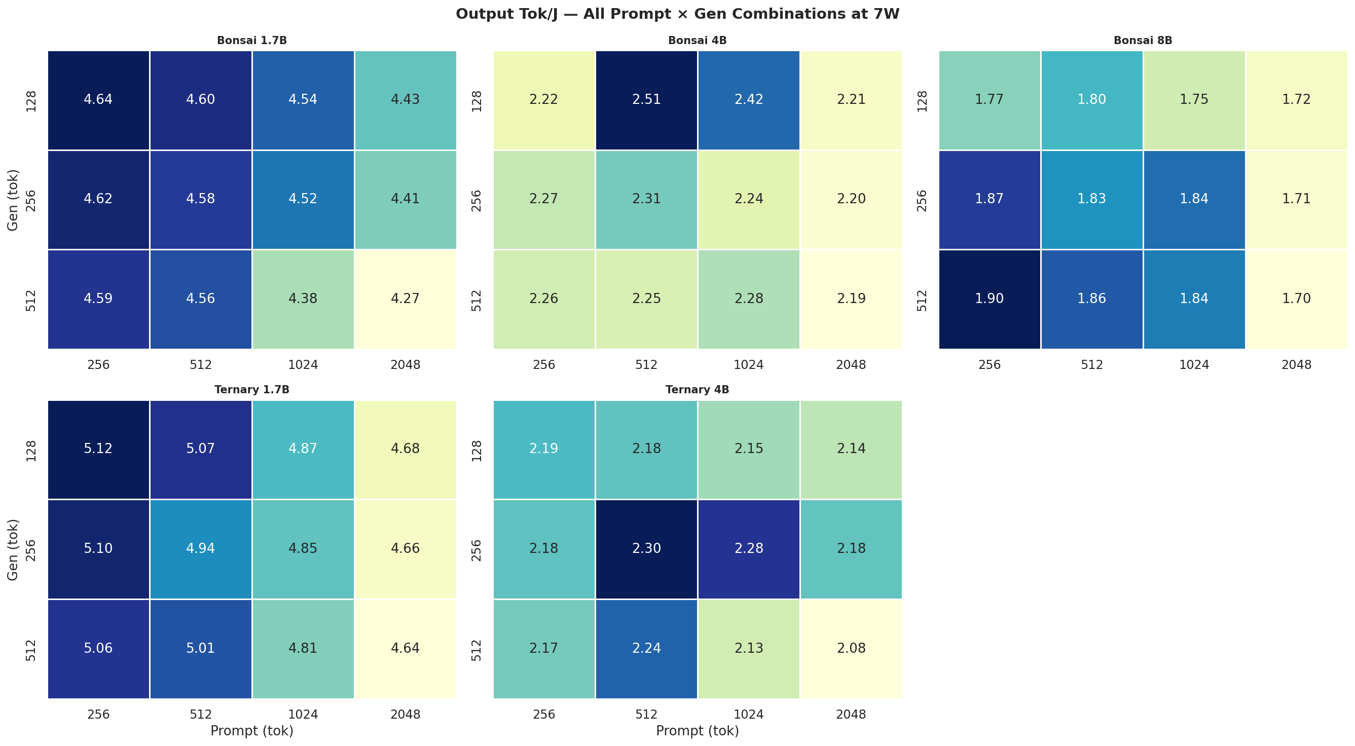
Figure C.2b: All 12 combos at 15W
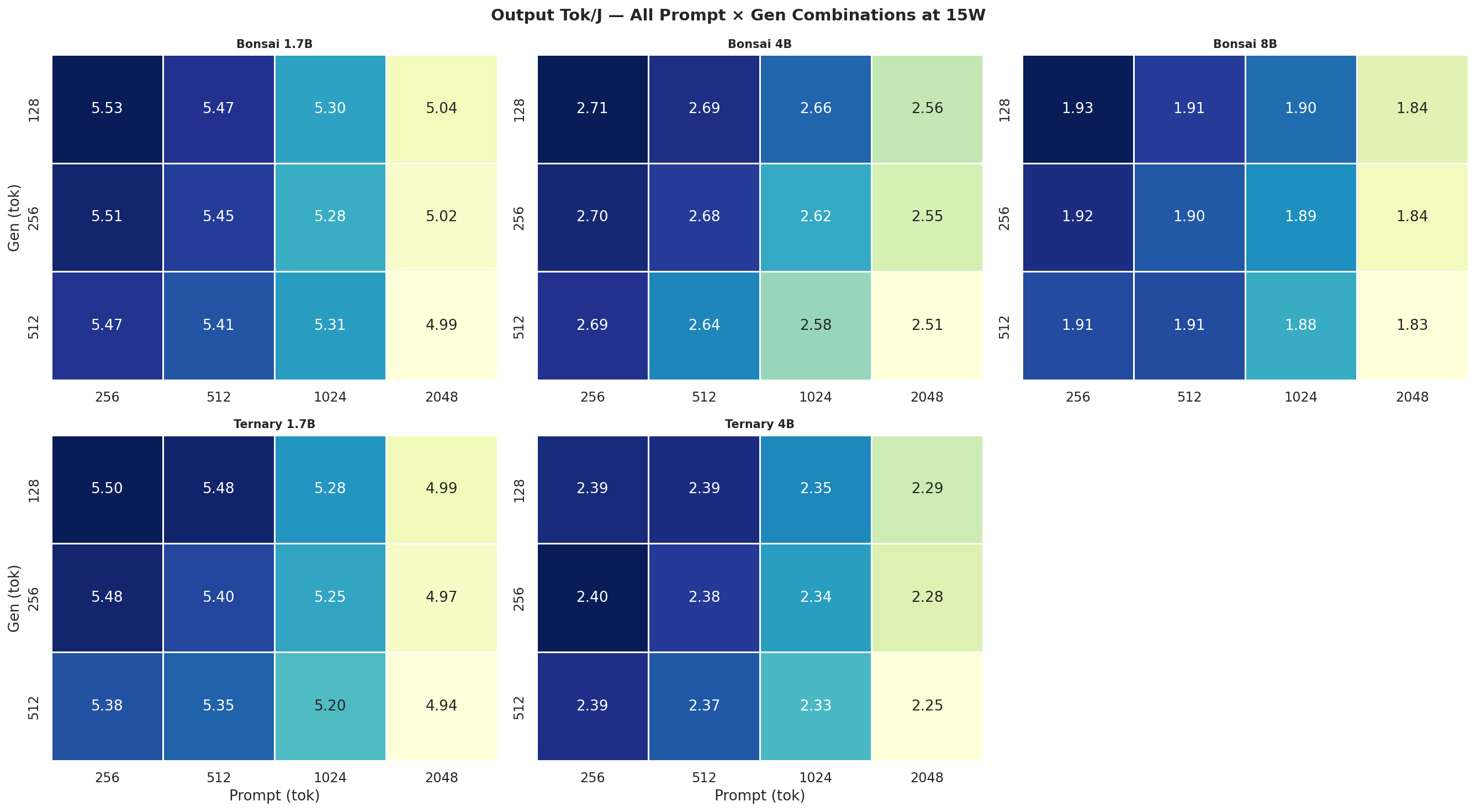
Figure C.2c: All 12 combos at 25W
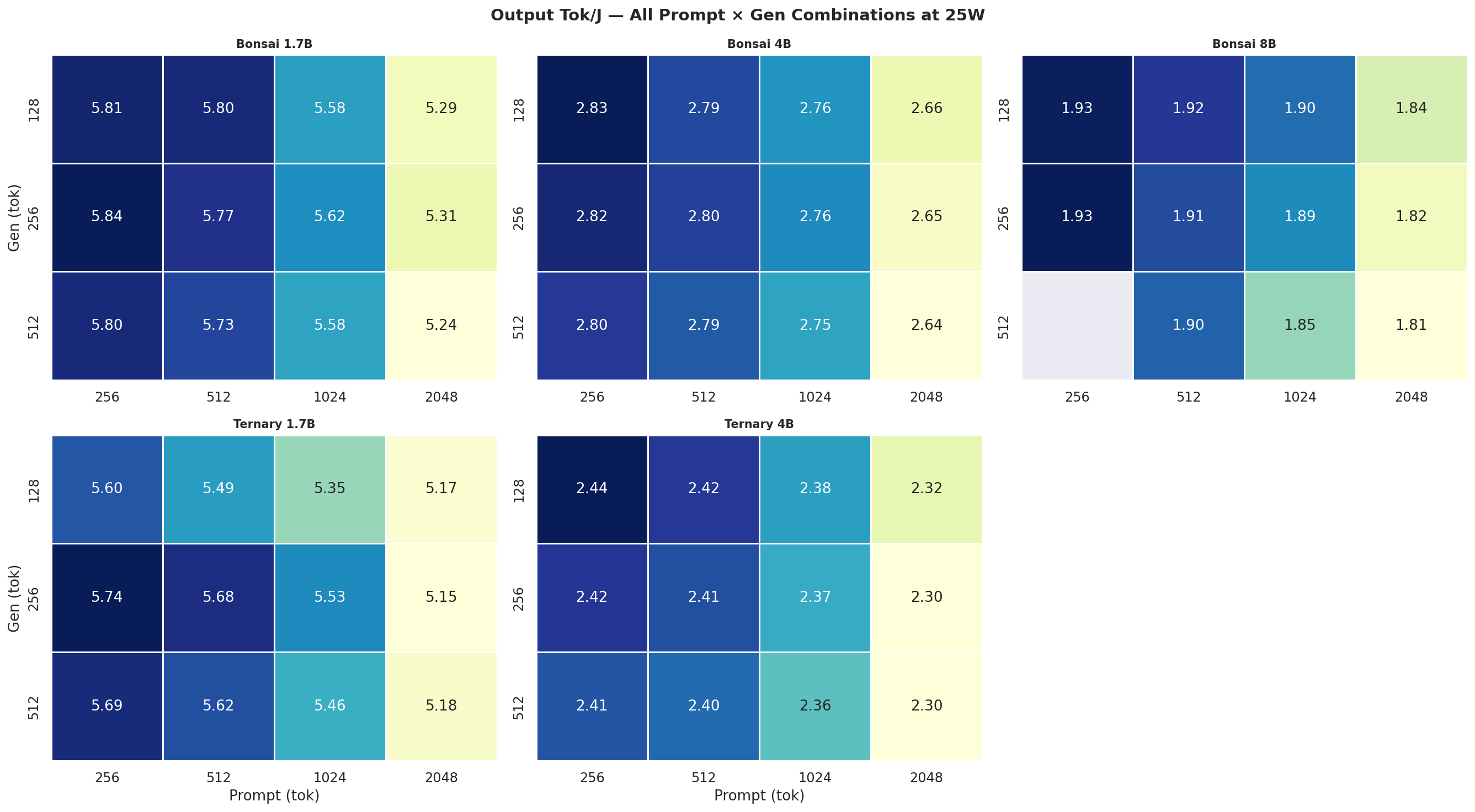
Figure C.2d: All 12 combos at MAXN
C.3 Phase power heatmaps (prefill and decode W)
Observed VDD_CPU_GPU_CV power during the prefill and decode phases separately, across all 12 prompt × gen combinations per power mode. Prefill is compute-heavy (batched forward pass); decode is memory-bandwidth bound (one token at a time) - the difference in watts between the two phases is visible in every mode.
Figure C.3a: Prefill power (W) at 7W
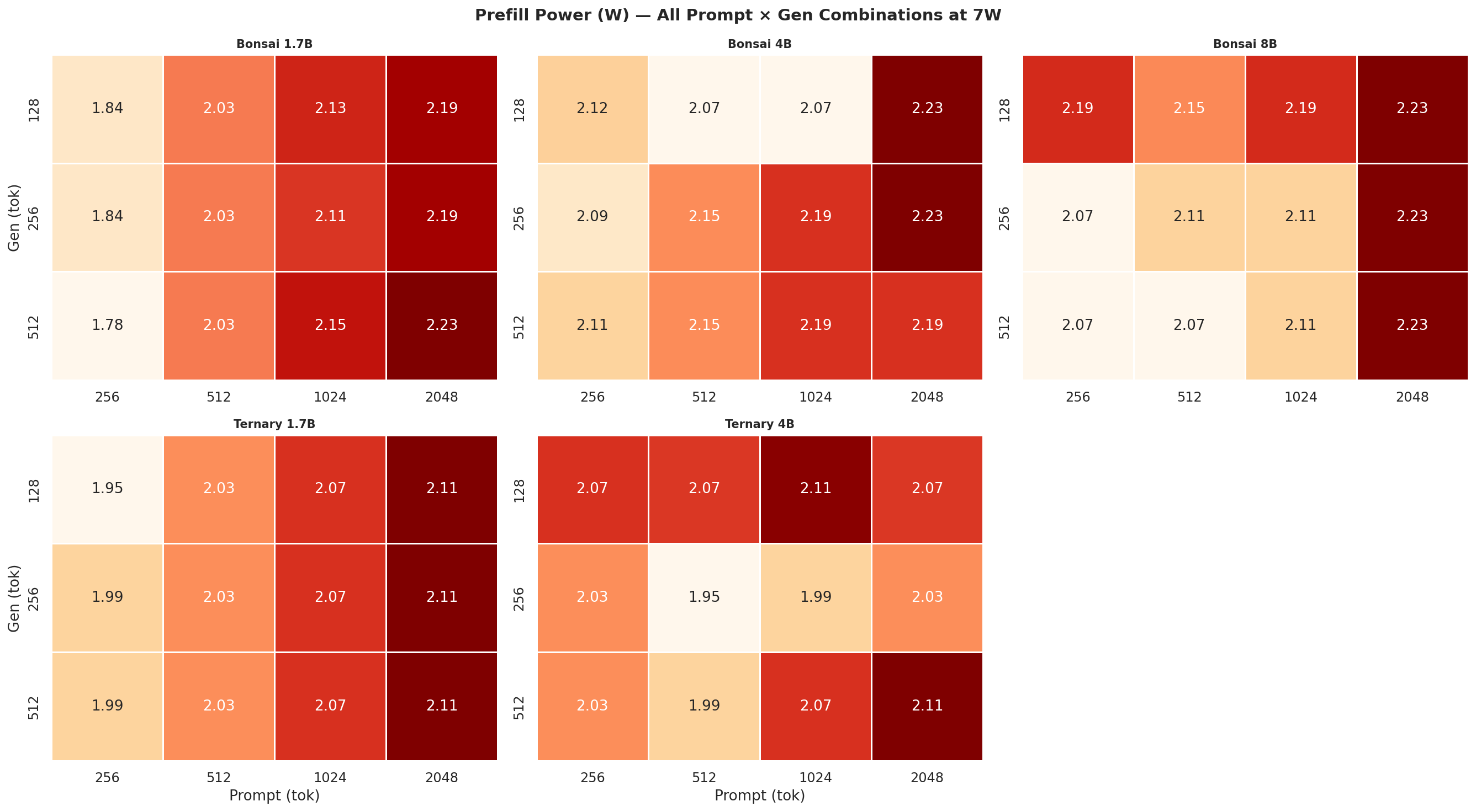
Figure C.3b: Prefill power (W) at 15W
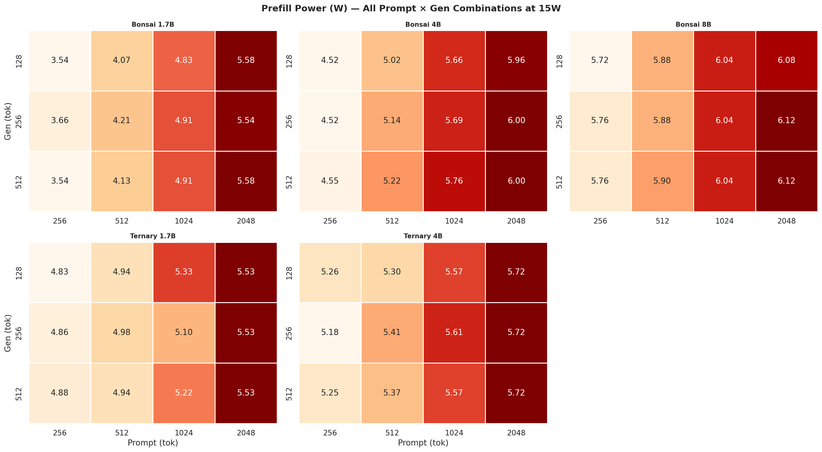
Figure C.3c: Prefill power (W) at 25W
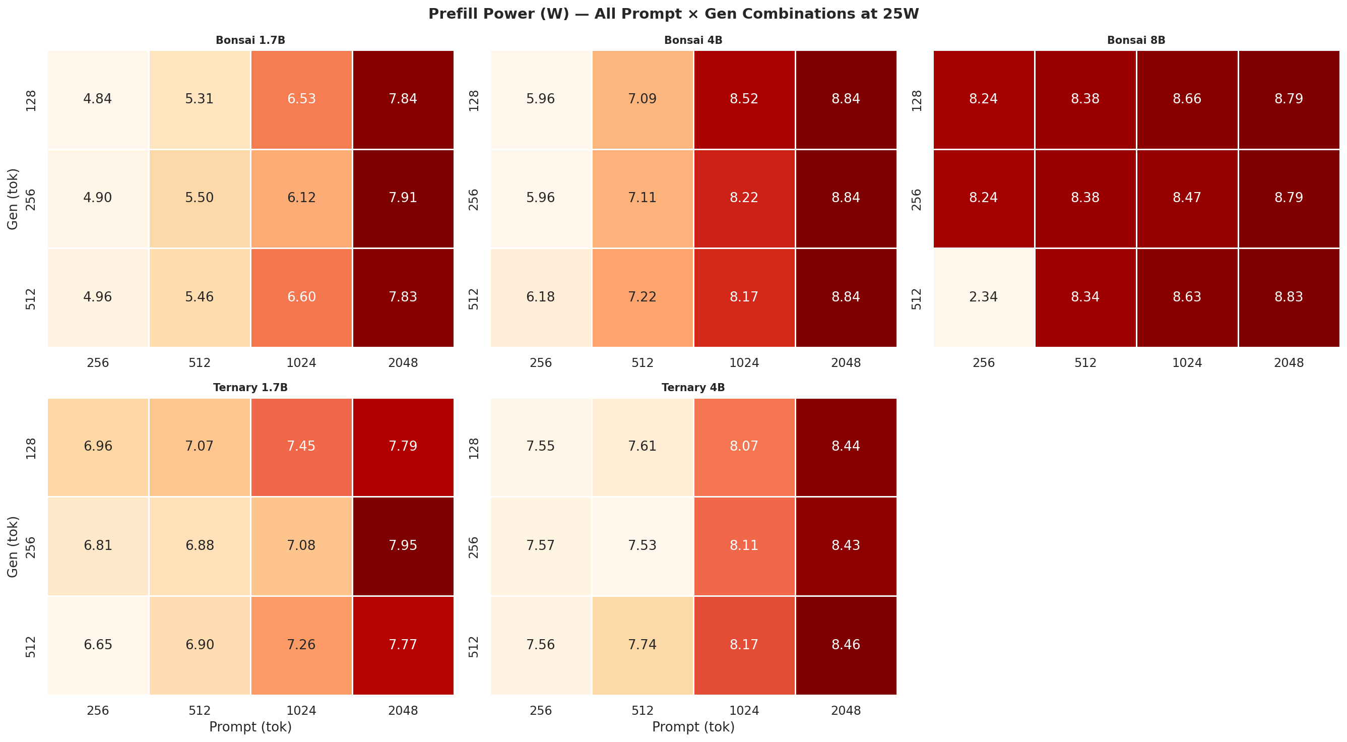
Figure C.3d: Prefill power (W) at MAXN
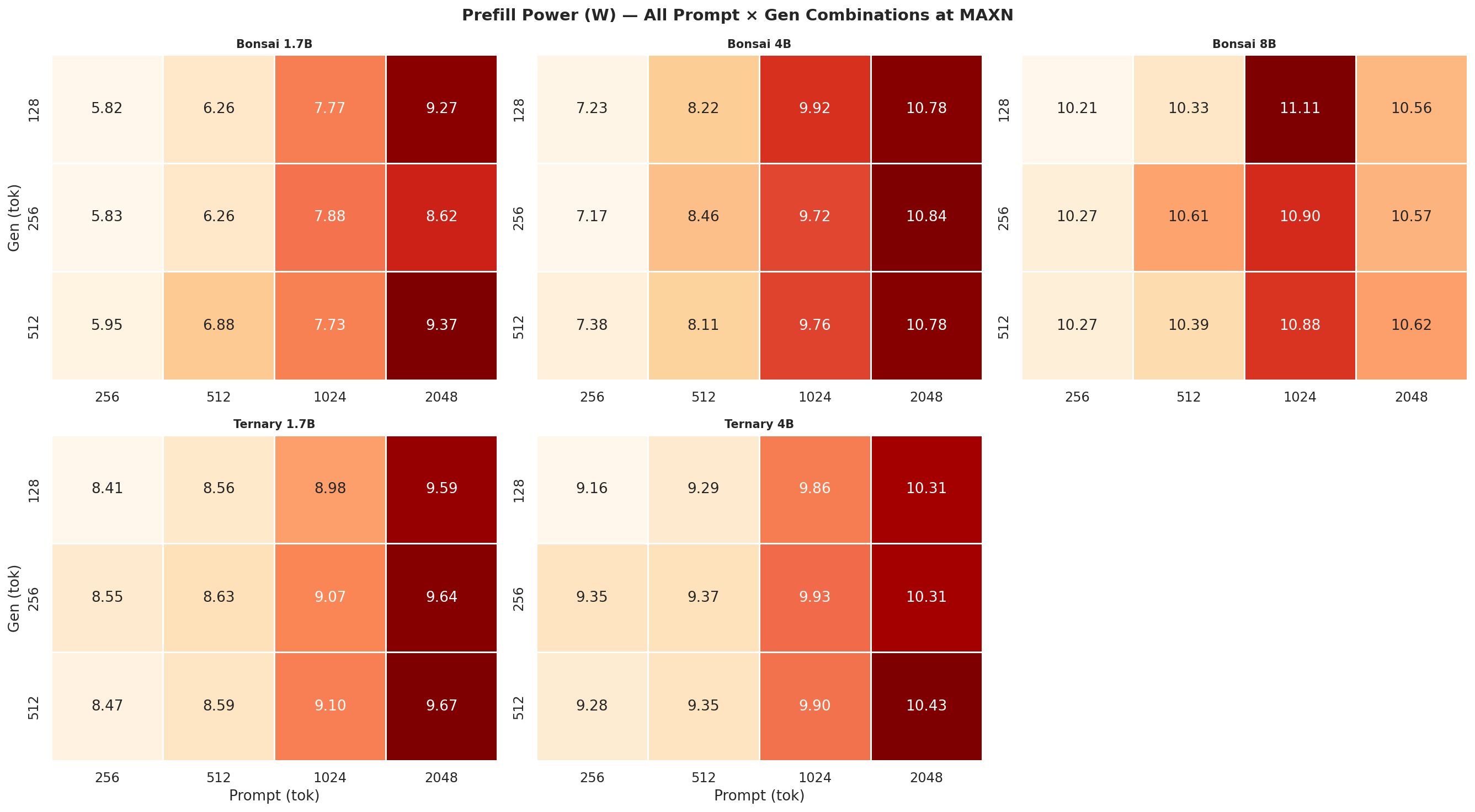
Figure C.3e: Decode power (W) at 7W
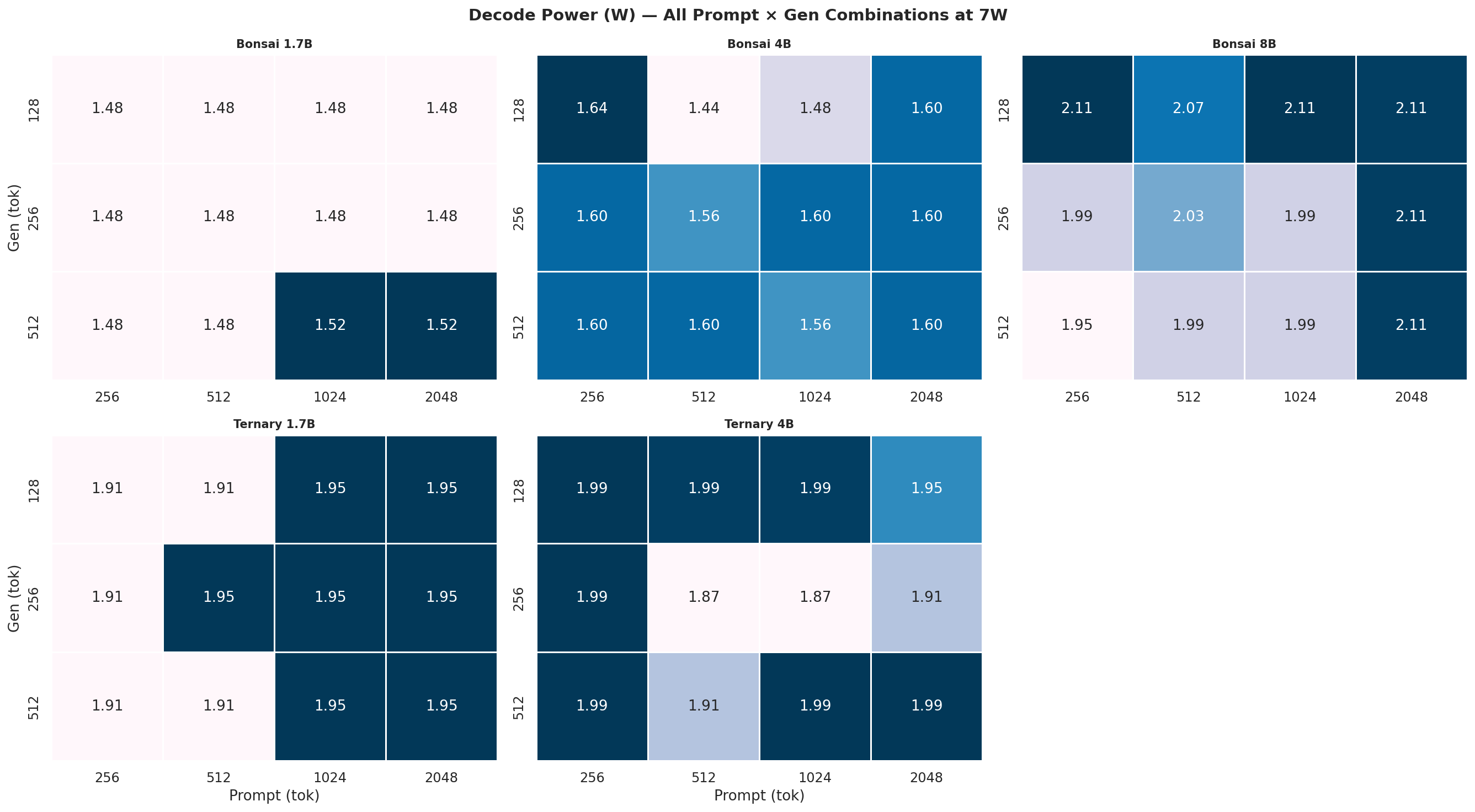
Figure C.3f: Decode power (W) at 15W
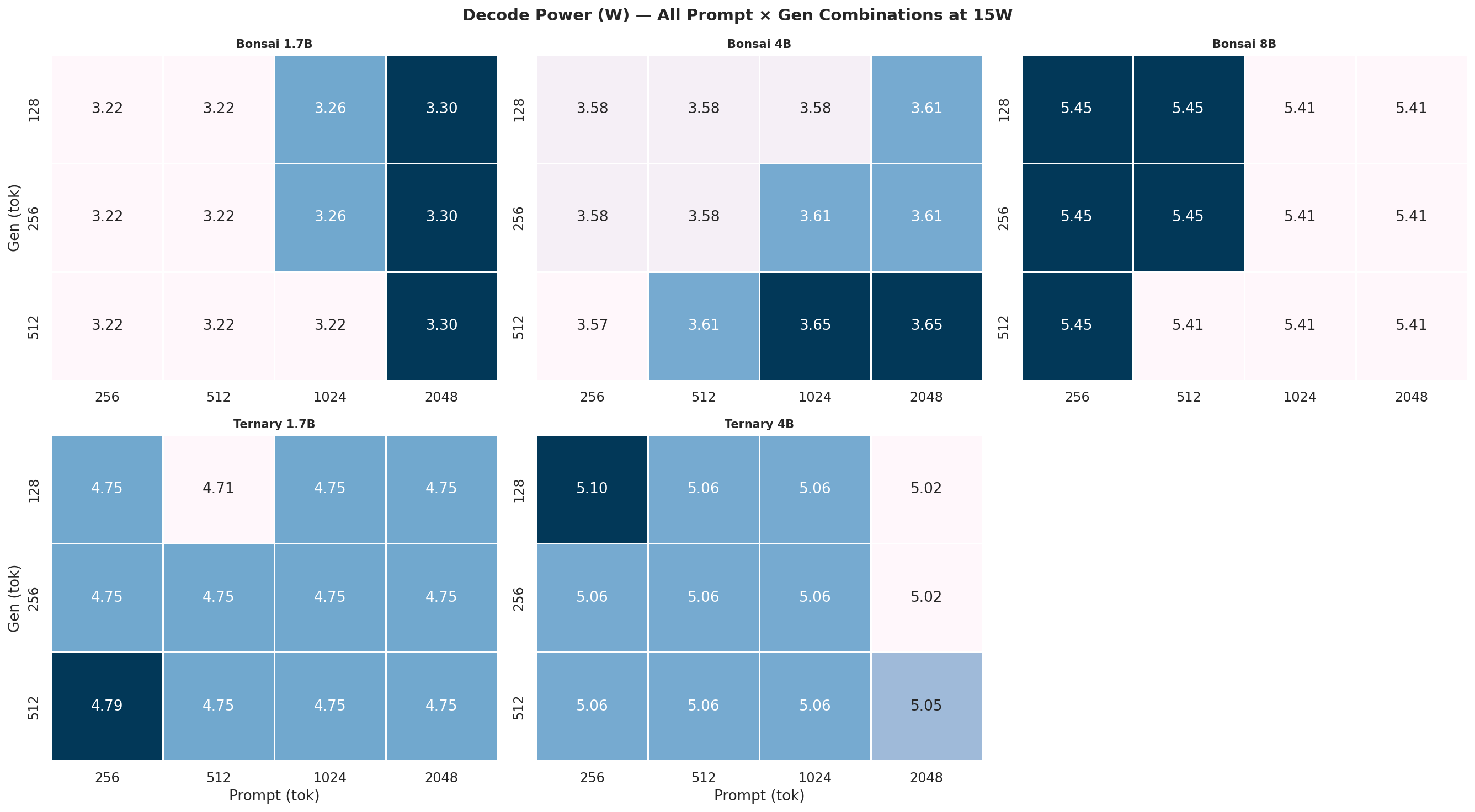
Figure C.3g: Decode power (W) at 25W
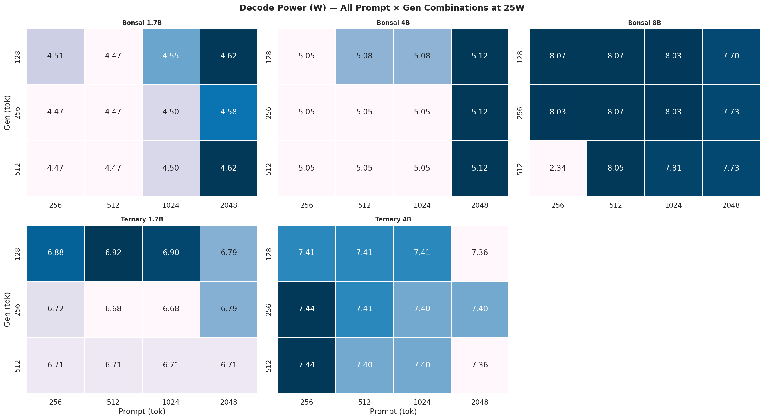
Figure C.3h: Decode power (W) at MAXN
Appendix D: Prefill / Decode / Total tok/J: All Combinations
All charts are 2×3 faceted line plots with a fixed y-scale across all subplots. The canonical combination (ctx=2048, gen=512) is also shown in §2.2.
D.1 Prefill tok/J (input tok / J) vs prompt length
Figure D.1a: Prefill tok/J vs prompt length: gen=128
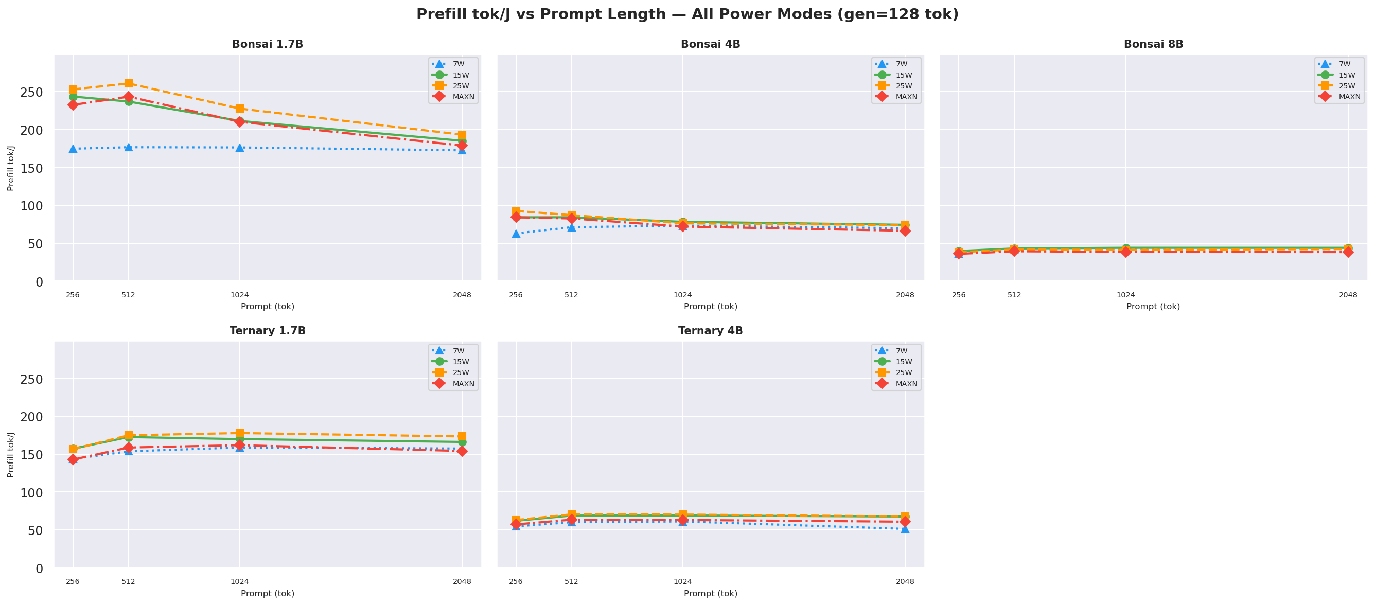
Figure D.1b: Prefill tok/J vs prompt length: gen=256

Figure D.1c: Prefill tok/J vs prompt length: gen=512 (canonical, also in § 2.2)
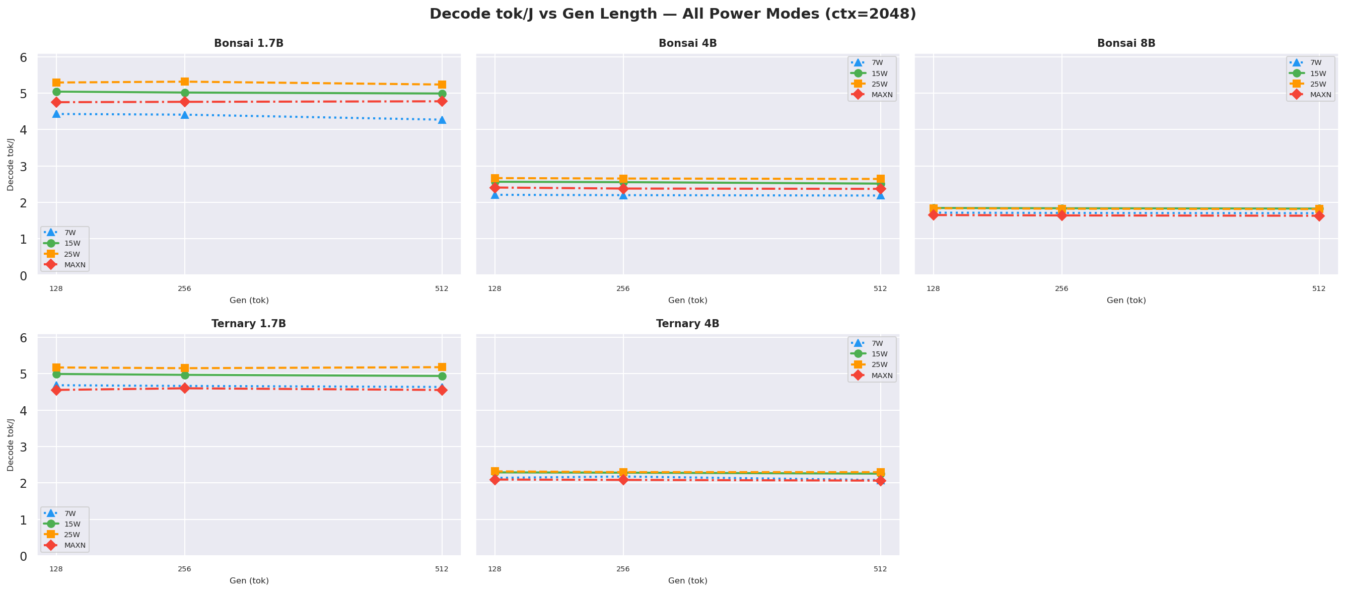
D.2 Decode tok/J (output tok / J) - independent of prompt length
Decode tok/J depends on the number of output tokens (gen length), not input prompt length, since decode happens after prefill completes. These charts show decode tok/J as a function of gen length for each prompt context length.
Figure D.2a: Decode tok/J vs gen length: ctx=256
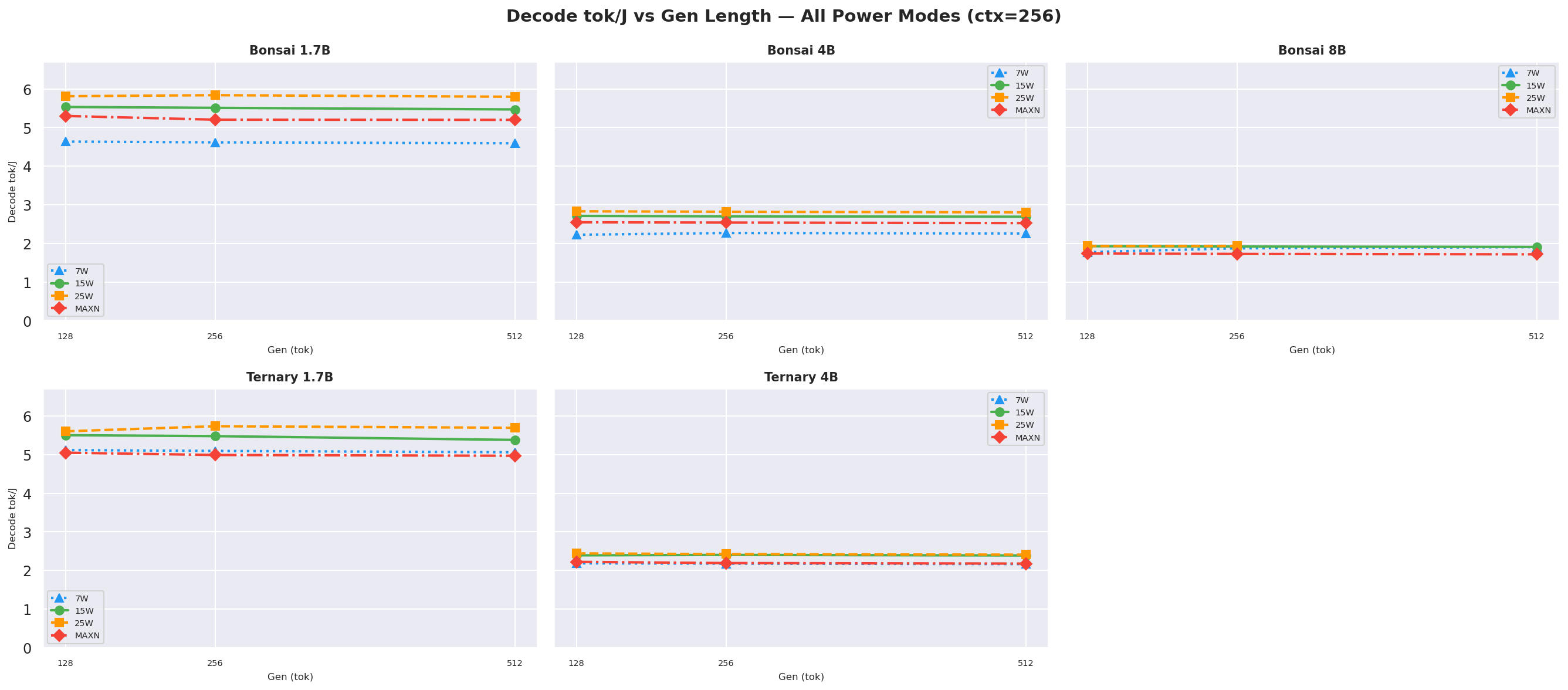
Figure D.2b: Decode tok/J vs gen length: ctx=512
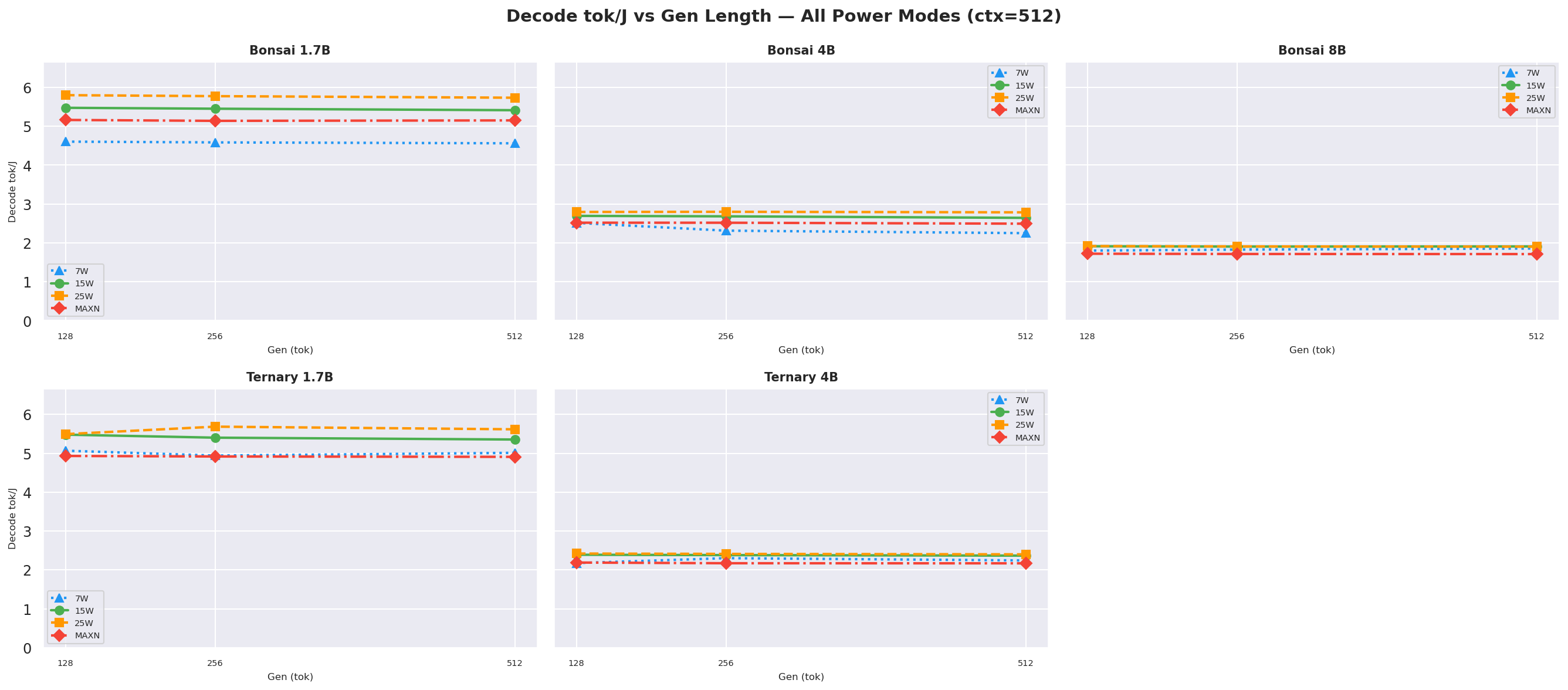
Figure D.2c: Decode tok/J vs gen length: ctx=1024
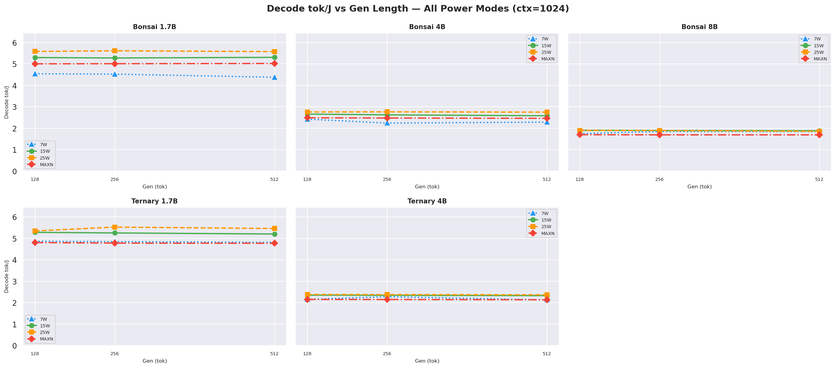
Figure D.2d: Decode tok/J vs gen length: ctx=2048
D.3 Total tok/J ((input+output) tok / J) vs prompt length
Figure D.3a: Total tok/J vs prompt length: gen=128
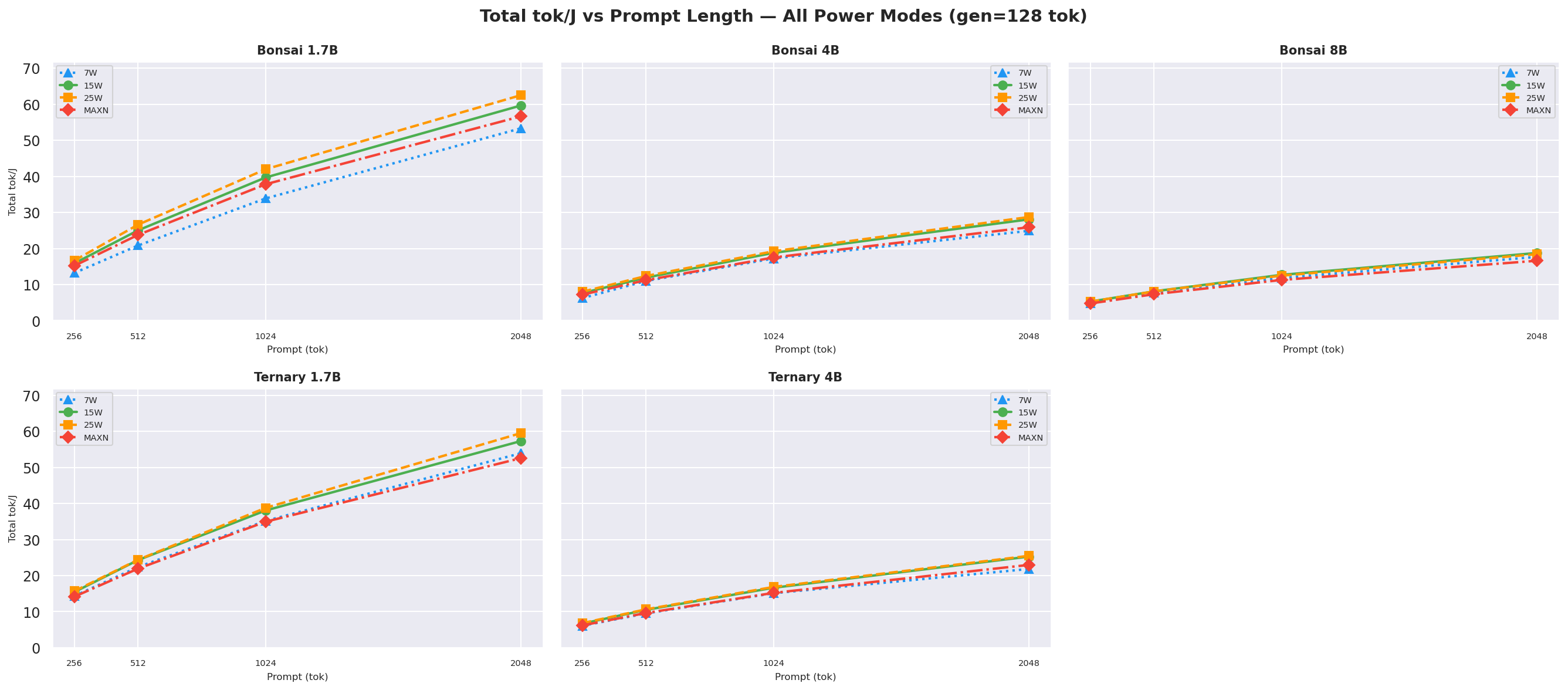
Figure D.3b: Total tok/J vs prompt length: gen=256
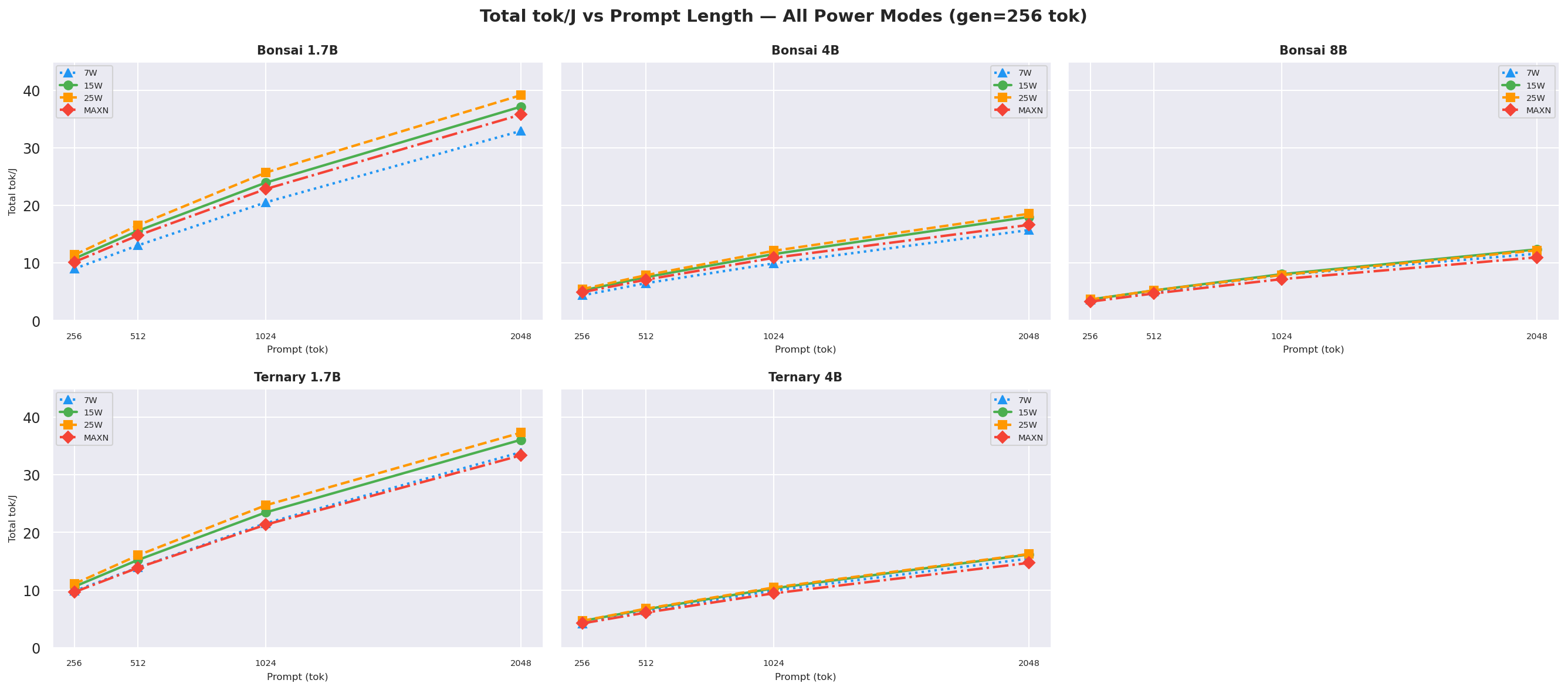
Figure D.3c: Total tok/J vs prompt length: gen=512 (canonical, also in § 2.2)
Appendix E: Latency: All Combinations
E.1 Request Latency (E2E)
Request latency (E2E) p50 - total time from request start to last token received. Line charts show variation with prompt length (2×3 facet, fixed y-scale).
E.1a Request latency vs prompt length (by gen length)
Figure E.1a: Request latency vs prompt length: gen=128
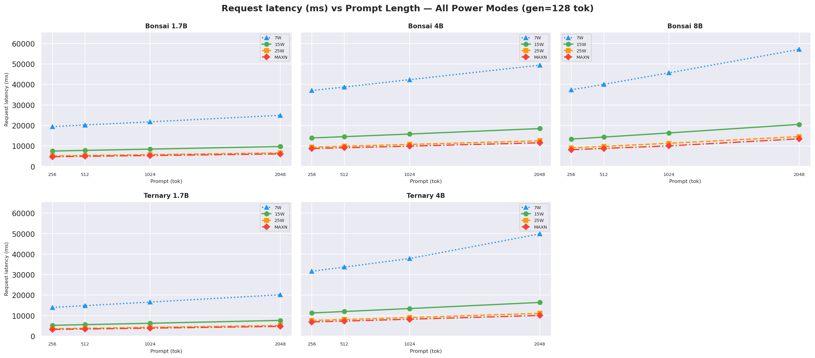
Figure E.1b: Request latency vs prompt length: gen=256
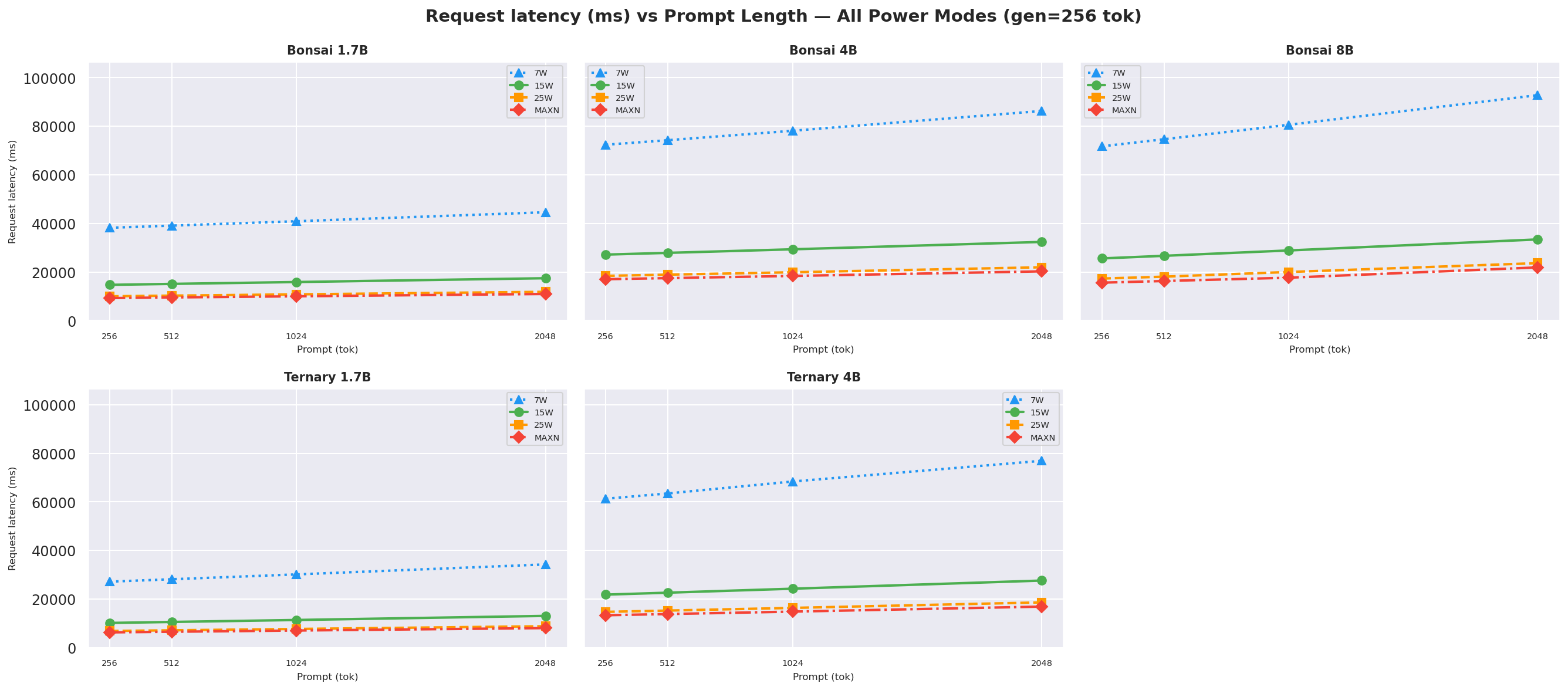
Figure E.1c: Request latency vs prompt length: gen=512 (canonical)
E.2 TTFT: All Prompt × Gen Combinations
TTFT p50 (median time to first token, ms) is driven almost entirely by prompt length - it is the prefill cost. These charts show how it varies across all 12 prompt × gen combinations and across all 4 power modes.
E.2a TTFT vs prompt length (by gen length)
Figure E.2a: TTFT vs prompt length: gen=128

Figure E.2b: TTFT vs prompt length: gen=256
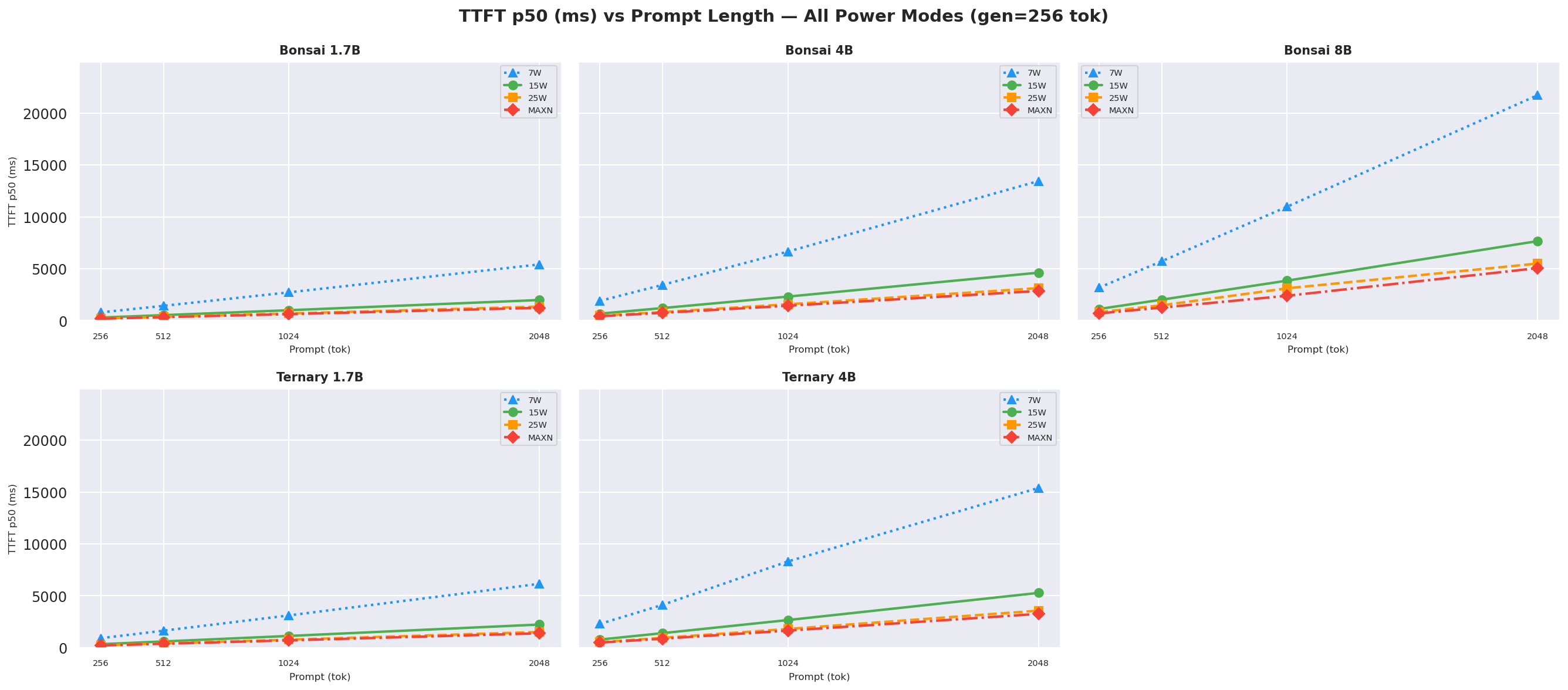
Figure E.2c: TTFT vs prompt length: gen=512 (canonical)
E.3 TTFT heatmaps (gen x prompt) per power mode
Each cell is TTFT in ms. Rows = gen length, columns = prompt length. Independent of gen length hence the same across rows.
Figure E.3a: TTFT heatmap: 7W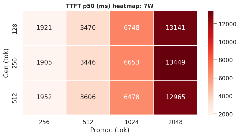
|
Figure E.3b: TTFT heatmap: 15W
|
Figure E.3c: TTFT heatmap: 25W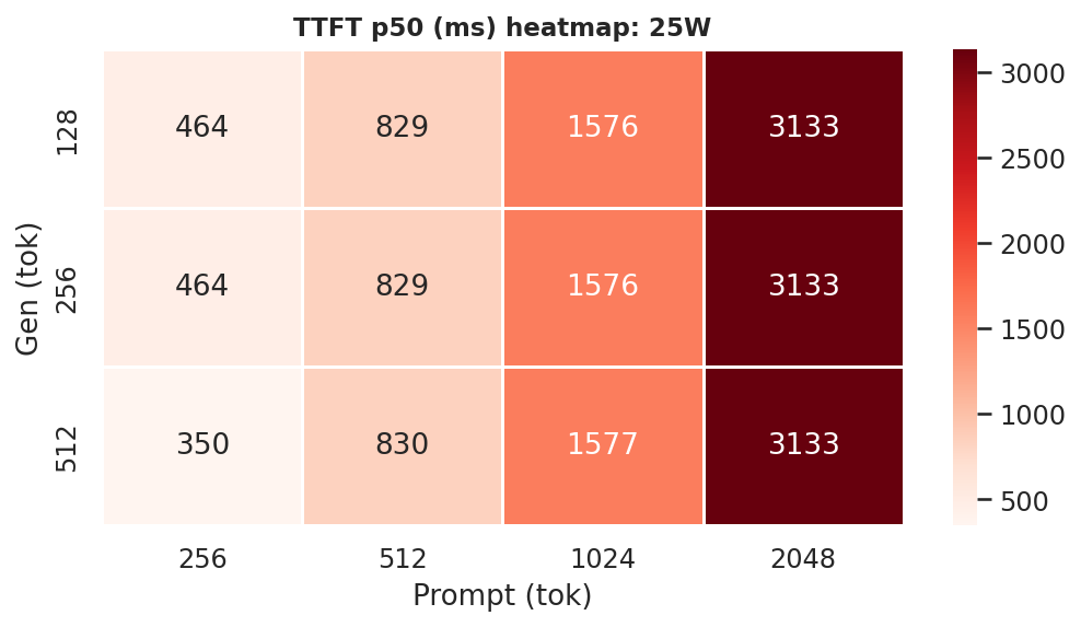
|
Figure E.3d: TTFT heatmap: MAXN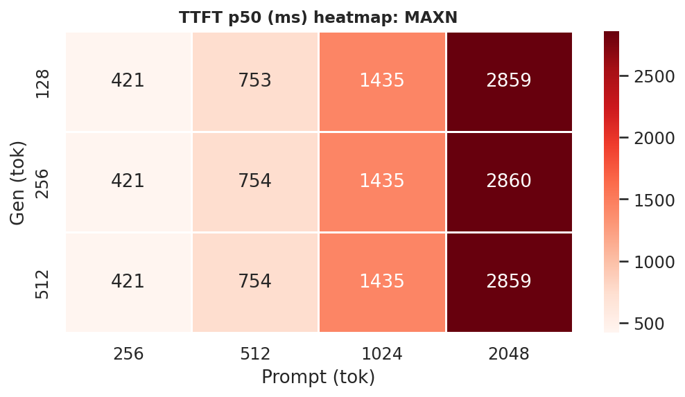
|
Appendix F: ITL: All Combinations
Inter-token latency (ms) = time between consecutive output tokens. It measures decode cost and is driven by model size and GPU clock, not prompt length.
F.1 ITL vs prompt length (by gen length)
Figure F.1a: ITL vs prompt length: gen=128
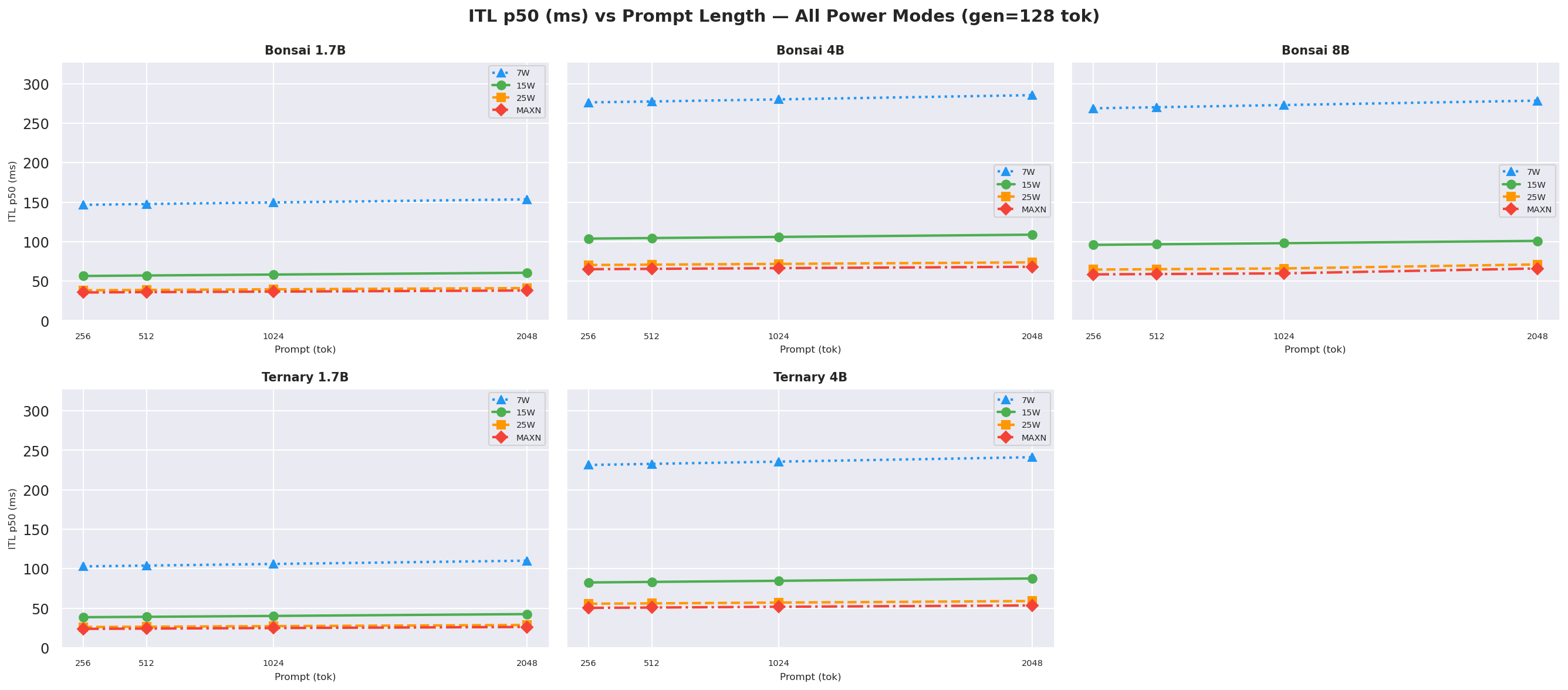
Figure F.1b: ITL vs prompt length: gen=256

Figure F.1c: ITL vs prompt length: gen=512 (canonical, also in section 2.3)
F.2 ITL heatmaps (gen x prompt) per power mode
Figure F.2a: ITL heatmap: 7W
|
Figure F.2b: ITL heatmap: 15W
|
Figure F.2c: ITL heatmap: 25W
|
Figure F.2d: ITL heatmap: MAXN
|
Appendix G: Prefill Throughput: All Combinations
Prefill throughput (tok/s) measures how fast the model processes input tokens. It scales with prompt length (longer prompts hit peak GPU utilisation) and GPU clock speed.
G.1 Prefill throughput vs prompt length (by gen length)
Figure G.1a: Prefill throughput vs prompt length: gen=128
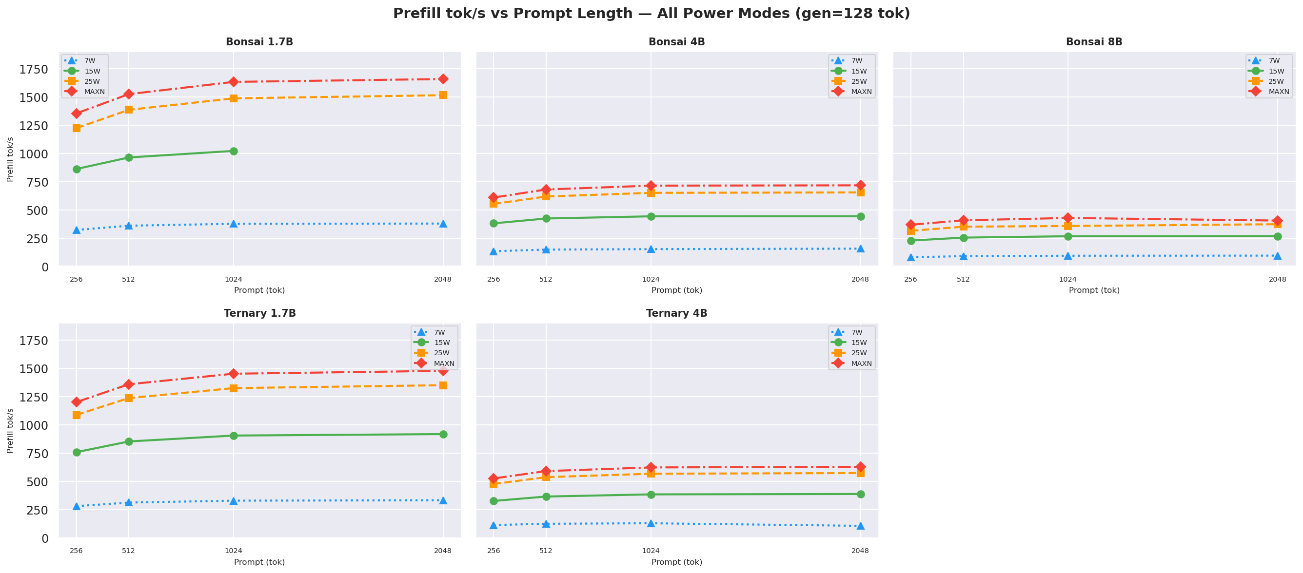
Figure G.1b: Prefill throughput vs prompt length: gen=256
Prefill throughput is independent of gen length, so gen=128 and gen=256 show the same trend.
G.2 Prefill throughput heatmaps (gen x prompt) per power mode
Figure G.2a: Prefill throughput heatmap: 7W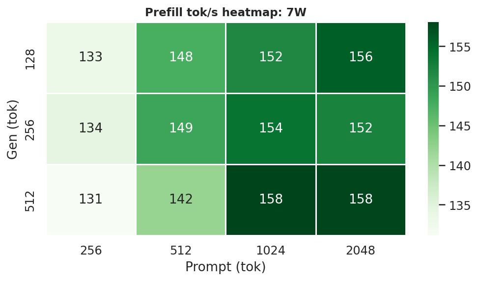
|
Figure G.2b: Prefill throughput heatmap: 15W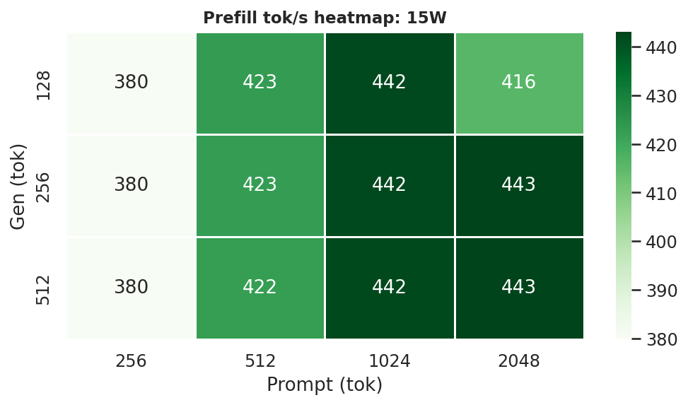
|
Figure G.2c: Prefill throughput heatmap: 25W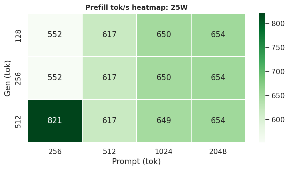
|
Figure G.2d: Prefill throughput heatmap: MAXN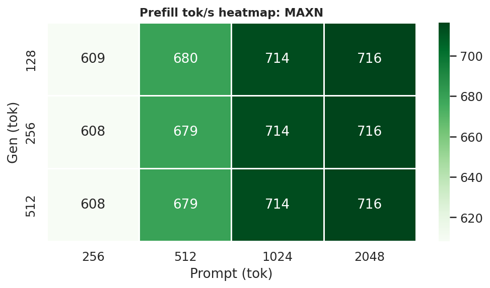
|
Appendix H: All Metrics, Formulas, and Calculation Methods
This appendix documents every metric reported in this benchmark, its formula, its source, and any caveats.
H.1 Raw inputs from aiperf and tegrastats
| Symbol | Source | Definition |
|---|---|---|
ISL |
aiperf JSON input_sequence_length.avg |
Actual input tokens processed per request (may differ from target due to tokenizer rounding) |
OSL |
aiperf JSON output_sequence_length.avg |
Actual output tokens generated per request |
TTFT |
aiperf JSON time_to_first_token.p50 (ms) |
Median time from request sent to first output token received; proxy for prefill duration. p50 used (not avg) to avoid skew from occasional slow requests |
ITL |
aiperf JSON inter_token_latency.p50 (ms) |
Median time between consecutive output tokens; per-token decode cost. p50 used for robustness against outliers |
RL |
aiperf JSON request_latency.p50 (ms) |
Median total wall time per request: TTFT + all inter-token intervals. p50 used for energy calculations |
tok_s |
aiperf JSON output_token_throughput_per_user.p50 |
Output tokens per second, single-user (OSL / RL in steady state) |
prefill_tput |
aiperf JSON prefill_throughput_per_user.p50 |
Input tokens processed per second during prefill phase |
t0, t1 |
aiperf JSON start_time, end_time (ISO 8601) |
Wall-clock start and end of the full 20-request profiling run |
mW_i |
tegrastats VDD_CPU_GPU_CV field (mW) |
Instantaneous power on the CPU+GPU+CV rail at sample i |
All aiperf metrics are averages over 20 requests per combo. Percentile variants (p50, p90, p99) are also available in the raw JSON but not reproduced here.
H.2 Power
p50_power_W = median(mW_i for all tegrastats samples where t0 <= sample_time <= t1) / 1000
VDD_CPU_GPU_CVcovers the CPU, GPU, and Computer Vision engine rail- Does NOT include board overhead (fan, storage, USB) which is on
VDD_IN VDD_INis ~1.5-3 W higher thanVDD_CPU_GPU_CVduring inference- Tegrastats interval: 500 ms
H.3 Output tok/J (main efficiency metric)
output_tok_J = OSL / decode_J
             = OSL / (decode_power_W * (RL_p50_s - TTFT_p50_s))
decode_power_W is the median power across tegrastats samples assigned to exact decode windows using per-request nanosecond timestamps from profile_export.jsonl (see H.5). The denominator is decode-phase energy only - prefill excluded because no output tokens are generated during prefill.
Higher is better. This is the primary metric of the benchmark.
Note: because decode time and decode power are both roughly independent of prompt length, output tok/J is also roughly independent of prompt length.
H.4 Request latency energy
total_J = p50_power_W * (RL_p50 / 1000)
Energy consumed by one median request from first byte sent to last token received. p50_power_W is the median tegrastats sample over the full run window. Accurate for all cells regardless of TTFT.
H.5 Prefill and decode energy
prefill_J  = prefill_power_W * (TTFT / 1000)
decode_J   = decode_power_W  * ((RL - TTFT) / 1000)
total_J    = prefill_J + decode_J

prefill_%  = prefill_J / total_J * 100
Exact per-request phase power from profile_export.jsonl. aiperf writes one JSON record per request to profile_export.jsonl, with nanosecond-precision timestamps:
request_start_ns  - when request was sent
request_ack_ns    - when first output token was received  (= prefill end)
request_end_ns    - when last output token was received   (= decode end)
For each request i, phase windows in wall-clock seconds are:
prefill_start_i = t0 + (request_start_ns_i - request_start_ns_0) / 1e9
prefill_end_i   = t0 + (request_ack_ns_i   - request_start_ns_0) / 1e9
decode_end_i    = t0 + (request_end_ns_i   - request_start_ns_0) / 1e9
where t0 is the aiperf start_time ISO timestamp and request_start_ns_0 is the first request’s start. Each tegrastats sample at wall-clock time ep is assigned to whichever request’s phase window it falls in.
prefill_power_W = median of samples in any prefill window across all 20 requests.
decode_power_W = median of samples in any decode window across all 20 requests.
Energy uses exact p50 (median) phase durations from the per-request data:
p50_ttft_s   = median(request_ack_ns_i - request_start_ns_i) / 1e9  over all 20 requests
p50_decode_s = median(request_end_ns_i - request_ack_ns_i)   / 1e9  over all 20 requests
Why this matters: prefill draws significantly more power than decode on Bonsai models - prefill is a batched forward pass (compute-heavy), decode is one token at a time (memory-bandwidth bound). At 25W the ratio is ~1.6x for 1.7B/4B models, ~1.1x for 8B. Using full-run average power for both phases would underestimate decode_power_W and therefore overestimate decode_J, making output_tok_J too low.
Residual approximation: a 500 ms tegrastats sample that straddles a prefill→decode boundary within a single request is assigned to one phase entirely. This affects only samples near the request_ack_ns boundary and is negligible across 20 requests totalling hundreds of samples.
H.6 Phase tok/J metrics
prefill_tok_J = ISL / prefill_J
              = ISL / (prefill_power_W * TTFT_s)

decode_tok_J  = OSL / decode_J
              = OSL / (decode_power_W * (RL_s - TTFT_s))

total_tok_J   = (ISL + OSL) / total_J
              = (ISL + OSL) / (prefill_J + decode_J)
Where TTFT_s = [TTFT](#glossary) / 1000, RL_s = RL / 1000.
prefill_tok_J: input tokens per joule of prefill energy, using phase-specificprefill_power_W.decode_tok_J: identical tooutput_tok_J- the primary benchmark metric, using phase-specificdecode_power_W.total_tok_J: all tokens (in + out) per joule of total request energy.
H.7 mJ per output token
mJ_per_output_tok = (decode_J / OSL) * 1000
                  = 1000 / decode_tok_J
Millijoules per generated output token (decode_J is in joules, ×1000 converts to mJ for readability). Carries the same caveat as I.5 for cells where TTFT < 500 ms.
H.8 Prefill throughput
prefill_tput (tok/s) = aiperf JSON prefill_throughput_per_user.p50
Directly from aiperf. Measures how fast input tokens are processed during the prefill phase. Scales with prompt length (longer prompts hit peak GPU utilisation) and GPU clock.
H.9 Speedup ratio methodology (Tables 9, 10a, 11, 12)
All speedup ratios use median over all 12 prompt × gen combos (4 ctx lengths × 3 gen lengths). “A vs B” means A is the faster mode; ratio > 1 means A is faster than B.
Table 9 - Output throughput (tok/s):
speedup_A_vs_B = median(tok_s_A  over 12 combos) / median(tok_s_B  over 12 combos)
tok_s = output_token_throughput_per_user.p50  (aiperf)
Table 10a - Decode time:
decode_time_s = (request_latency.p50 - time_to_first_token.p50) / 1000
speedup_A_vs_B = median(decode_time_s_B over 12 combos) / median(decode_time_s_A over 12 combos)
Table 11 - TTFT (prefill time):
speedup_A_vs_B = median(TTFT_B over 12 combos) / median(TTFT_A over 12 combos)
TTFT = time_to_first_token.p50  (aiperf, ms)
Table 12 - Request latency (E2E):
speedup_A_vs_B = median(RL_B over 12 combos) / median(RL_A over 12 combos)
RL = request_latency.p50  (aiperf, ms)
H.10 Best total tok/J per model (Table 13)
best_total_tok_J(model) = max(total_tok_J(mode, model, gen, ctx))
                          over all modes in {7W, 15W, 25W, MAXN}
                          and all gen in {128, 256, 512}
                          and all ctx in {256, 512, 1024, 2048}

total_tok_J = (ISL + OSL) / (p50_power_W * RL_p50_s)
The single highest total tok/J value observed for that model across all 48 combinations. Peaks at ctx=2048, gen=128 for every model because the long prompt dominates the (ISL + OSL) numerator.
H.11 TTFT, ITL, RL percentiles
All percentile variants come directly from aiperf JSON without further computation:
TTFT       = time_to_first_token.p50   (canonical; p50 used everywhere)
TTFT_p90   = time_to_first_token.p90
TTFT_p99   = time_to_first_token.p99
ITL        = inter_token_latency.p50    (canonical; p50 used everywhere)
ITL_p99    = inter_token_latency.p99
RL         = request_latency.p50        (canonical; p50 used everywhere)
RL_p99     = request_latency.p99
H.12 Energy caveat: which metrics are accurate vs approximate
| Metric | Accurate? | Condition |
|---|---|---|
output_tok_J |
Always | No phase split needed |
total_J |
Always | Full window power * RL |
decode_J |
Mostly | avg_power approx decode power since decode dominates window |
decode_tok_J |
Mostly | Same as above |
total_tok_J |
Always | Uses total_J which is accurate |
prefill_J |
TTFT >= 500 ms only |
Needs tegrastats sample in prefill window |
prefill_tok_J |
TTFT >= 500 ms only |
Derived from prefill_J |
prefill_% |
TTFT >= 500 ms only |
Derived from prefill_J |
mJ_per_output_tok |
Mostly | Derived from decode_J |
Phase energies use phase-specific power from tegrastats samples assigned to exact prefill/decode windows via per-request nanosecond timestamps from profile_export.jsonl (see I.5). The residual approximation is only the few tegrastats samples that straddle a phase boundary near each request’s TTFT transition - negligible across 20 requests. output_tok_J is computable for 239 of 240 cells; the one exception (Bonsai-8B / 25W / ctx=256 / gen=512) is a complete benchmark failure - all 20 aiperf requests errored - unrelated to power measurement.
H.13 Power and temperature
p50_power_W = median(tegrastats.VDD_CPU_GPU_CV[mW] / 1000
               for all samples where aiperf_t0 <= sample_time <= aiperf_t1)
Power is the median VDD_CPU_GPU_CV (CPU+GPU+CV rail) from tegrastats sampled at 500 ms intervals, over each model’s active inference window only (idle/cool-down between models excluded). Median is used instead of mean to suppress rare outlier samples (e.g. OS scheduling spikes) that do not reflect sustained inference power.
Junction temperature (TJ) is the hottest internal die temperature on the Jetson SoC, reported by tegrastats as tj@. The hardware automatically throttles GPU/CPU clocks when TJ reaches ~95 °C to prevent damage. Peak TJ < 76 °C across all runs confirms ample thermal headroom at every power mode.
| Symbol | Source | Definition |
|---|---|---|
VDD_CPU_GPU_CV |
tegrastats | Instantaneous power (mW) on the CPU+GPU+CV rail |
cpu@ |
tegrastats | CPU cluster temperature (°C) |
gpu@ |
tegrastats | GPU temperature (°C) |
tj@ |
tegrastats | Junction (hottest internal die) temperature (°C) |
p50_power_W |
computed | Median VDD_CPU_GPU_CV over active inference window (W) |
avg_cpu_C |
computed | Mean CPU temp over active inference window |
avg_gpu_C |
computed | Mean GPU temp over active inference window |
peak_tj_C |
computed | Maximum TJ temperature observed |
Throttling is flagged when peak_tj_C > 85 °C (leaving a 10 °C safety margin below the hardware limit).
Appendix I: All ctx x gen Combinations - tok/s and tok/J
Full breakdown of output tok/s and output tok/J for all 5 models across all 4 power modes, repeated for every combination of prompt context length (ctx) and generation length (gen). Each table mirrors Table 7 (the canonical ctx=2048, gen=512 cell) but at a different operating point.
Bold values indicate the peak tok/J mode for that model row; when two modes tie on tok/J (to 2 decimal places), the higher-throughput mode is bolded. All values use p50 (median) over 20 requests.
gen=128 tok
Table I.1: ctx=256, gen=128
| Model | 7W tok/s | 15W tok/s | 25W tok/s | MAXN tok/s | 7W tok/J | 15W tok/J | 25W tok/J | MAXN tok/J | Peak tok/J |
|---|---|---|---|---|---|---|---|---|---|
| Bonsai-1.7B | 6.8 | 17.7 | 26.0 | 28.0 | 4.64 | 5.53 | 5.81 | 5.30 | 25W |
| Bonsai-4B | 3.6 | 9.6 | 14.2 | 15.3 | 2.22 | 2.71 | 2.83 | 2.55 | 25W |
| Bonsai-8B | 3.7 | 10.4 | 15.5 | 17.1 | 1.77 | 1.93 | 1.93 | 1.74 | 25W |
| Ternary-Bonsai-1.7B | 9.7 | 25.9 | 38.2 | 41.9 | 5.12 | 5.50 | 5.60 | 5.05 | 25W |
| Ternary-Bonsai-4B | 4.3 | 12.1 | 18.0 | 19.8 | 2.19 | 2.39 | 2.44 | 2.22 | 25W |
Table I.2: ctx=512, gen=128
| Model | 7W tok/s | 15W tok/s | 25W tok/s | MAXN tok/s | 7W tok/J | 15W tok/J | 25W tok/J | MAXN tok/J | Peak tok/J |
|---|---|---|---|---|---|---|---|---|---|
| Bonsai-1.7B | 6.8 | 17.5 | 25.7 | 27.7 | 4.60 | 5.47 | 5.80 | 5.16 | 25W |
| Bonsai-4B | 3.6 | 9.6 | 14.1 | 15.2 | 2.51 | 2.69 | 2.79 | 2.52 | 25W |
| Bonsai-8B | 3.7 | 10.3 | 15.3 | 16.9 | 1.80 | 1.91 | 1.92 | 1.72 | 25W |
| Ternary-Bonsai-1.7B | 9.6 | 25.6 | 37.7 | 41.3 | 5.07 | 5.48 | 5.49 | 4.93 | 25W |
| Ternary-Bonsai-4B | 4.3 | 12.0 | 17.8 | 19.7 | 2.18 | 2.39 | 2.42 | 2.19 | 25W |
Table I.3: ctx=1024, gen=128
| Model | 7W tok/s | 15W tok/s | 25W tok/s | MAXN tok/s | 7W tok/J | 15W tok/J | 25W tok/J | MAXN tok/J | Peak tok/J |
|---|---|---|---|---|---|---|---|---|---|
| Bonsai-1.7B | 6.7 | 17.1 | 25.2 | 27.2 | 4.54 | 5.30 | 5.58 | 5.00 | 25W |
| Bonsai-4B | 3.6 | 9.4 | 13.9 | 15.0 | 2.42 | 2.66 | 2.76 | 2.48 | 25W |
| Bonsai-8B | 3.7 | 10.2 | 15.1 | 16.7 | 1.75 | 1.90 | 1.90 | 1.70 | 25W |
| Ternary-Bonsai-1.7B | 9.4 | 24.9 | 36.6 | 40.2 | 4.87 | 5.28 | 5.35 | 4.80 | 25W |
| Ternary-Bonsai-4B | 4.2 | 11.8 | 17.5 | 19.3 | 2.15 | 2.35 | 2.38 | 2.15 | 25W |
Table I.4: ctx=2048, gen=128
| Model | 7W tok/s | 15W tok/s | 25W tok/s | MAXN tok/s | 7W tok/J | 15W tok/J | 25W tok/J | MAXN tok/J | Peak tok/J |
|---|---|---|---|---|---|---|---|---|---|
| Bonsai-1.7B | 6.5 | 16.5 | 24.3 | 26.2 | 4.43 | 5.04 | 5.29 | 4.75 | 25W |
| Bonsai-4B | 3.5 | 9.2 | 13.5 | 14.7 | 2.21 | 2.56 | 2.66 | 2.41 | 25W |
| Bonsai-8B | 3.6 | 9.9 | 14.0 | 15.1 | 1.72 | 1.84 | 1.84 | 1.65 | 25W |
| Ternary-Bonsai-1.7B | 9.1 | 23.5 | 34.8 | 38.1 | 4.68 | 4.99 | 5.17 | 4.55 | 25W |
| Ternary-Bonsai-4B | 4.1 | 11.4 | 16.9 | 18.7 | 2.14 | 2.29 | 2.32 | 2.09 | 25W |
gen=256 tok
Table I.5: ctx=256, gen=256
| Model | 7W tok/s | 15W tok/s | 25W tok/s | MAXN tok/s | 7W tok/J | 15W tok/J | 25W tok/J | MAXN tok/J | Peak tok/J |
|---|---|---|---|---|---|---|---|---|---|
| Bonsai-1.7B | 6.8 | 17.7 | 26.0 | 28.0 | 4.62 | 5.51 | 5.84 | 5.20 | 25W |
| Bonsai-4B | 3.6 | 9.6 | 14.2 | 15.3 | 2.27 | 2.70 | 2.82 | 2.54 | 25W |
| Bonsai-8B | 3.7 | 10.4 | 15.5 | 17.1 | 1.87 | 1.92 | 1.93 | 1.73 | 25W |
| Ternary-Bonsai-1.7B | 9.7 | 25.9 | 38.4 | 41.9 | 5.10 | 5.48 | 5.74 | 4.99 | 25W |
| Ternary-Bonsai-4B | 4.3 | 12.1 | 18.0 | 19.8 | 2.18 | 2.40 | 2.42 | 2.19 | 25W |
Table I.6: ctx=512, gen=256
| Model | 7W tok/s | 15W tok/s | 25W tok/s | MAXN tok/s | 7W tok/J | 15W tok/J | 25W tok/J | MAXN tok/J | Peak tok/J |
|---|---|---|---|---|---|---|---|---|---|
| Bonsai-1.7B | 6.8 | 17.5 | 25.7 | 27.7 | 4.58 | 5.45 | 5.77 | 5.14 | 25W |
| Bonsai-4B | 3.6 | 9.6 | 14.1 | 15.2 | 2.31 | 2.68 | 2.80 | 2.52 | 25W |
| Bonsai-8B | 3.7 | 10.3 | 15.3 | 16.9 | 1.83 | 1.90 | 1.91 | 1.71 | 25W |
| Ternary-Bonsai-1.7B | 9.6 | 25.5 | 37.8 | 41.3 | 4.94 | 5.40 | 5.68 | 4.92 | 25W |
| Ternary-Bonsai-4B | 4.3 | 12.0 | 17.8 | 19.6 | 2.30 | 2.38 | 2.41 | 2.17 | 25W |
Table I.7: ctx=1024, gen=256
| Model | 7W tok/s | 15W tok/s | 25W tok/s | MAXN tok/s | 7W tok/J | 15W tok/J | 25W tok/J | MAXN tok/J | Peak tok/J |
|---|---|---|---|---|---|---|---|---|---|
| Bonsai-1.7B | 6.7 | 17.1 | 25.2 | 27.2 | 4.52 | 5.28 | 5.62 | 5.01 | 25W |
| Bonsai-4B | 3.6 | 9.4 | 13.9 | 15.0 | 2.24 | 2.62 | 2.76 | 2.47 | 25W |
| Bonsai-8B | 3.7 | 10.2 | 15.1 | 16.7 | 1.84 | 1.89 | 1.89 | 1.69 | 25W |
| Ternary-Bonsai-1.7B | 9.4 | 24.8 | 36.8 | 40.1 | 4.85 | 5.25 | 5.53 | 4.78 | 25W |
| Ternary-Bonsai-4B | 4.2 | 11.8 | 17.5 | 19.3 | 2.28 | 2.34 | 2.37 | 2.14 | 25W |
Table I.8: ctx=2048, gen=256
| Model | 7W tok/s | 15W tok/s | 25W tok/s | MAXN tok/s | 7W tok/J | 15W tok/J | 25W tok/J | MAXN tok/J | Peak tok/J |
|---|---|---|---|---|---|---|---|---|---|
| Bonsai-1.7B | 6.5 | 16.5 | 24.3 | 26.2 | 4.41 | 5.02 | 5.31 | 4.76 | 25W |
| Bonsai-4B | 3.5 | 9.2 | 13.5 | 14.6 | 2.20 | 2.55 | 2.65 | 2.38 | 25W |
| Bonsai-8B | 3.6 | 9.9 | 14.0 | 15.1 | 1.71 | 1.84 | 1.82 | 1.64 | 15W |
| Ternary-Bonsai-1.7B | 9.1 | 23.5 | 34.8 | 38.2 | 4.66 | 4.97 | 5.15 | 4.60 | 25W |
| Ternary-Bonsai-4B | 4.1 | 11.4 | 16.9 | 18.7 | 2.18 | 2.28 | 2.30 | 2.08 | 25W |
gen=512 tok
Table I.9: ctx=256, gen=512
| Model | 7W tok/s | 15W tok/s | 25W tok/s | MAXN tok/s | 7W tok/J | 15W tok/J | 25W tok/J | MAXN tok/J | Peak tok/J |
|---|---|---|---|---|---|---|---|---|---|
| Bonsai-1.7B | 6.8 | 17.6 | 25.9 | 27.9 | 4.59 | 5.47 | 5.80 | 5.20 | 25W |
| Bonsai-4B | 3.6 | 9.6 | 14.1 | 15.3 | 2.26 | 2.69 | 2.80 | 2.53 | 25W |
| Bonsai-8B | 3.7 | 10.4 | - | 17.0 | 1.90 | 1.91 | - | 1.72 | 15W |
| Ternary-Bonsai-1.7B | 9.7 | 25.7 | 38.1 | 41.7 | 5.06 | 5.38 | 5.69 | 4.97 | 25W |
| Ternary-Bonsai-4B | 4.3 | 12.1 | 17.9 | 19.7 | 2.17 | 2.39 | 2.41 | 2.18 | 25W |
Table I.10: ctx=512, gen=512
| Model | 7W tok/s | 15W tok/s | 25W tok/s | MAXN tok/s | 7W tok/J | 15W tok/J | 25W tok/J | MAXN tok/J | Peak tok/J |
|---|---|---|---|---|---|---|---|---|---|
| Bonsai-1.7B | 6.7 | 17.4 | 25.6 | 27.6 | 4.56 | 5.41 | 5.73 | 5.15 | 25W |
| Bonsai-4B | 3.6 | 9.5 | 14.0 | 15.2 | 2.25 | 2.64 | 2.79 | 2.49 | 25W |
| Bonsai-8B | 3.7 | 10.3 | 15.3 | 16.9 | 1.86 | 1.91 | 1.90 | 1.71 | 15W |
| Ternary-Bonsai-1.7B | 9.6 | 25.4 | 37.6 | 41.1 | 5.01 | 5.35 | 5.62 | 4.91 | 25W |
| Ternary-Bonsai-4B | 4.3 | 12.0 | 17.7 | 19.6 | 2.24 | 2.37 | 2.40 | 2.17 | 25W |
Table I.11: ctx=1024, gen=512
| Model | 7W tok/s | 15W tok/s | 25W tok/s | MAXN tok/s | 7W tok/J | 15W tok/J | 25W tok/J | MAXN tok/J | Peak tok/J |
|---|---|---|---|---|---|---|---|---|---|
| Bonsai-1.7B | 6.7 | 17.1 | 25.0 | 27.1 | 4.38 | 5.31 | 5.58 | 5.02 | 25W |
| Bonsai-4B | 3.6 | 9.4 | 13.9 | 15.0 | 2.28 | 2.58 | 2.75 | 2.46 | 25W |
| Bonsai-8B | 3.7 | 10.2 | 14.4 | 16.6 | 1.84 | 1.88 | 1.85 | 1.69 | 15W |
| Ternary-Bonsai-1.7B | 9.4 | 24.6 | 36.6 | 40.0 | 4.81 | 5.20 | 5.46 | 4.77 | 25W |
| Ternary-Bonsai-4B | 4.2 | 11.7 | 17.4 | 19.2 | 2.13 | 2.33 | 2.36 | 2.13 | 25W |
Table I.12: ctx=2048, gen=512
| Model | 7W tok/s | 15W tok/s | 25W tok/s | MAXN tok/s | 7W tok/J | 15W tok/J | 25W tok/J | MAXN tok/J | Peak tok/J | |
|---|---|---|---|---|---|---|---|---|---|---|
| Bonsai-1.7B | 6.5 | 16.4 | 24.1 | 26.1 | 4.27 | 4.99 | 5.24 | 4.77 | 25W | |
| Bonsai-4B | 3.5 | 9.2 | 13.5 | 14.6 | 2.19 | 2.51 | 2.64 | 2.37 | 25W | |
| Bonsai-8B | 3.6 | 9.9 | 14.0 | 15.1 | 1.70 | 1.83 | 1.81 | 1.63 | 15W | |
| Ternary-Bonsai-1.7B | 9.0 | 23.4 | 34.7 | 38.0 | 4.64 | 4.94 | 5.18 | 4.55 | 25W | |
| Ternary-Bonsai-4B | 4.1 | 11.4 | 16.9 | 18.6 | 2.08 | 2.25 | 2.30 | 2.06 | 25W | — |
Trivia: Why Ternary Beats 1-bit on Jetson Despite Being Larger
Running the ternary models faster than the Q1_0 Bonsai models seems counterintuitive: ternary weights are stored at 2 bits each (4 per byte) while Q1_0 is 1 bit each (8 per byte), so Q1_0 has a smaller file and less DRAM pressure per decode step. Yet ternary wins on every mode. Here is why.
Storage vs compute type are separate things.
| Format | Storage | Compute path | Tensor core support on GA10B |
|---|---|---|---|
| Ternary {-1, 0, +1} | 2 bits/weight | unpack to INT8, use INT8 WMMA | Yes |
| Q1_0 {-1, +1} | 1 bit/weight | needs XNOR+popcount (BMMA / INT1) | No |
True 1-bit compute uses XNOR + popcount via BMMA instructions. XOR the packed weight bits with packed activation bits, then count the ones with popcount. Extremely fast when supported. NVIDIA added INT1 tensor cores (BMMA) on A100 (GA100) and select Turing chips. The Jetson Orin Nano runs the GA10B Ampere die, which does not include BMMA. So Q1_0 falls back to slow CUDA core emulation.
Ternary unpacks to INT8 {-1, 0, 1}, and INT8 WMMA tensor cores are present on GA10B. Ternary gets hardware-accelerated matmul; Q1_0 does not.
Zero-weight sparsity is a second real advantage. BitNet 1.58 models carry roughly 30-50% zero weights. Those accumulations are skipped entirely, saving a genuine fraction of flops even in the FP16/INT8 accumulation path. Q1_0 binary weights have no zeros, so there is no sparsity to exploit.
What good 1-bit kernels would look like. A proper XNOR+popcount kernel on hardware that supports BMMA would in theory beat ternary: smaller DRAM footprint AND fast bitwise arithmetic. The reason 1-bit loses here is not an inherent property of 1-bit quantization – it is a hardware availability gap on this specific Jetson die, combined with immature llama.cpp kernel support for Q1_0.
Kernel quality is about more than the arithmetic. Even when the per-weight operation is just add/subtract, the CUDA kernel controls: memory coalescing (whether 32 warp threads read contiguous addresses into a single DRAM transaction or scatter into 32 separate ones); shared memory tiling (loading weight blocks into fast on-chip SRAM before accumulation vs hitting DRAM on every access); warp divergence from the zero-weight skip (a naive if/skip branch serializes the warp – a good kernel uses predicated execution or precomputed bitmasks); and occupancy (register pressure determines how many warps stay in flight to hide memory latency). The arithmetic is one clock cycle. Everything around it determines whether the GPU is actually executing that cycle or stalling.
⚠ Why Models with Weights > ~1 GB Were Not Tested (and even so with higher ctx/gen lengths)
All models in this benchmark have GGUF weights ≤ 958 MB. Larger models (e.g. Gemma3-4B Q4_K_M at 2.4 GB) fail to load on JetPack R36.4.7 (L4T 36.4) regardless of power mode or available memory. This is a known regression in the CUDA IOVA / NvMap contiguous-memory allocator introduced in this JetPack release - not a simple “out of RAM” failure.
Root cause: On Jetson platforms, the CUDA driver allocates device-mapped memory through the
NvMapkernel driver, which requires a single contiguous block in the IOVA (I/O Virtual Address) space. Unlike a general-purpose allocator that can stitch together scattered pages, NvMap must find one unbroken IOVA range large enough for the entire allocation in a single call. For a 2.4 GB GGUF like Gemma3-4B, that means requesting a contiguous block of roughly 2.4 GB (plus KV-cache and CUDA runtime overhead) before any other tensor or buffer is placed in the address space.The allocation fails immediately with
NvMapMemAllocInternalTagged: error 12 (ENOMEM)- errno 12 isENOMEM, “not enough memory” in the contiguous-mapping sense, not the total-capacity sense.What this means in practice: Any GGUF model requiring more than roughly 1.1 GB of contiguous CUDA buffers is blocked at load time on this JetPack version. This is why the benchmark is limited to models under ~1 GB GGUF size. Smaller models load fine because their contiguous IOVA requirement fits within what the fragmented address space can still provide.
Affected platform: NVIDIA Jetson Orin Nano Super 8GB running JetPack R36.4.7 (L4T 36.4.7 / Ubuntu 22.04). The same board on JetPack 6.2.2 (L4T 36.5) resolves this regression.